GWAS with masreml
📐 Theory: Theory overview
This tutorial runs an EMMAX-style mixed-model GWAS with masreml, inspects the results, validates them against the bundled ground-truth QTL positions, and feeds them into GWABLUP — the GWAS-assisted re-weighting of the GRM that lifts GBLUP accuracy when the trait has a non-infinitesimal component. The full code is adapted from masreml/examples/04_gwas.R.
Setup
SNP-based GWAS
Step 1 — Fit the mixed model
run_gwas() consumes a fitted masreml object: it pulls variance components and the genomic relationship matrix from there. Fit the baseline GBLUP first.
Code
y_snp <- setNames(d$pheno$y_cont_qtl_snp, ids)
W_snp <- d$snp
storage.mode(W_snp) <- "double"
rownames(W_snp)     <- ids

fit_snp_g <- masreml(
  y       = y_snp,
  markers = list(snp_add = W_snp),
  method  = "auto",
  trait   = "continuous",
  verbose = FALSE
)
summary(fit_snp_g)
══ masreml Summary ═══════════════════════════════════

Model:
  Call            : masreml(y = y_snp, markers = list(snp_add = W_snp), method = "auto",
   Call            :     trait = "continuous", verbose = FALSE)
  Individuals     : 200
  Components      : snp_add, residual
  Log-likelihood  : -142.2201
  Algorithm       : AI
  Solver          : cholesky
  Converged       : TRUE (iterations = 9)

Variance Components:
 Component   Sigma2     H2 Proportion
   snp_add 0.627084 0.3669     0.3669
  residual 1.081864     NA     0.6331

Training Performance:
  accuracy (r)    : 0.7887
  R^2             : 0.6221
  RMSE            : 0.9054
  bias (slope)    : 1.594

GEBV Summary:
 Component     Min Mean    Max     SD
   snp_add -1.4617    0 1.4869 0.6592
     total -1.4617    0 1.4869 0.6592

══════════════════════════════════════════════════════
Step 2 — Run the GWAS scan
Code
List of 10
 $ lr         : num [1:500] 0.06719 0.00144 0.00103 0.0521 0.01003 ...
 $ beta       : num [1:500] -0.03012 0.00373 0.00616 0.02683 0.01199 ...
 $ se         : num [1:500] 0.0822 0.0694 0.136 0.0831 0.0846 ...
 $ pval       : num [1:500] 0.714 0.957 0.964 0.747 0.887 ...
 $ smoothed_lr: num [1:500] 0.0232 0.0304 0.0264 0.0317 0.0317 ...
 $ pp         : num [1:500] 0.00102 0.00103 0.00103 0.00103 0.00103 ...
 $ marker_type: chr "snp"
 $ n_markers  : int 500
 $ pi         : num 0.001
 $ window     : int 5
 - attr(*, "class")= chr "gwas_result"
The output is a list with per-marker columns including:
-
pval— frequentist \(p\) from the EMMAX-style score test -
pp— Bayesian model-averaged posterior probability of non-zero effect (used by GWABLUP for re-weighting) - effect estimates and likelihood ratios
Step 3 — Top peaks
Code
top10_snp_idx <- order(-gwas_snp$pp)[seq_len(10L)]
kable(data.frame(
  SNP   = map_snp$SNP[top10_snp_idx],
  CHROM = map_snp$CHROM[top10_snp_idx],
  POS   = map_snp$POS[top10_snp_idx],
  pval  = signif(gwas_snp$pval[top10_snp_idx], 3),
  pp    = round(gwas_snp$pp[top10_snp_idx], 3)
), caption = "Top 10 SNPs ranked by posterior probability (pp)")| SNP | CHROM | POS | pval | pp |
|---|---|---|---|---|
| SNP372 | 4 | 8100000 | 0.48200 | 0.003 |
| SNP371 | 4 | 8000000 | 0.85200 | 0.003 |
| SNP094 | 1 | 10300000 | 0.29800 | 0.003 |
| SNP090 | 1 | 9900000 | 0.89400 | 0.002 |
| SNP091 | 1 | 10000000 | 0.88200 | 0.002 |
| SNP092 | 1 | 10100000 | 0.00555 | 0.002 |
| SNP093 | 1 | 10200000 | 0.99100 | 0.002 |
| SNP029 | 1 | 3800000 | 0.01150 | 0.002 |
| SNP028 | 1 | 3700000 | 0.76600 | 0.002 |
| SNP356 | 4 | 6500000 | 0.48700 | 0.002 |
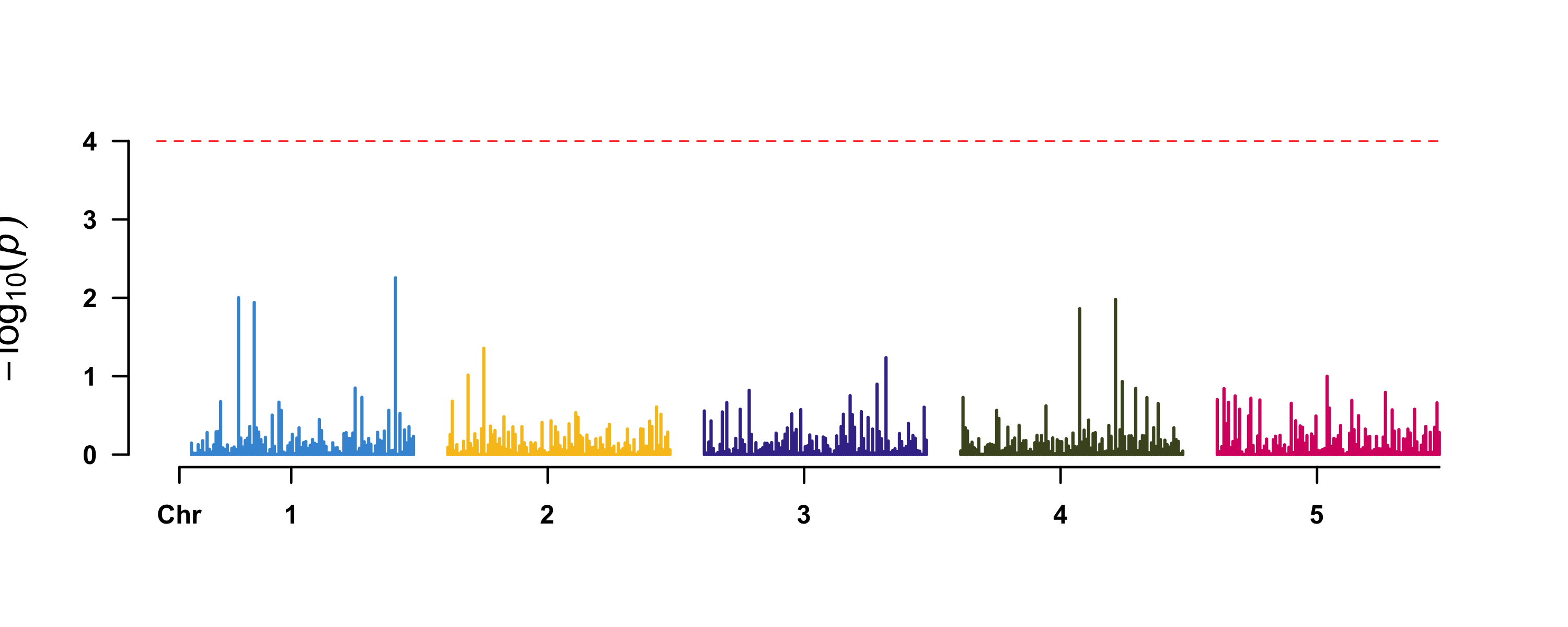
Step 4 — Manhattan plot (\(-\log_{10}(p)\))
CMplot (Yin et al.) provides publication-quality genome-wide plots with chromosome banding and threshold lines. We render in-chunk via file.output = FALSE.
Code
pval_cap <- 1e-12
thr_snp_p <- 0.05 / n_snp

snp_pval_df <- data.frame(
  SNP  = map_snp$SNP,
  Chr  = map_snp$CHROM,
  Pos  = map_snp$POS,
  pval = pmax(gwas_snp$pval, pval_cap),
  check.names = FALSE
)
snp_pval_hl <- as.character(map_snp$SNP[gwas_snp$pval < thr_snp_p])
if (length(snp_pval_hl) == 0L) snp_pval_hl <- NULL

CMplot::CMplot(
  snp_pval_df,
  type           = "h",
  plot.type      = "m",
  LOG10          = TRUE,
  threshold      = thr_snp_p,
  threshold.lty  = 2,
  threshold.lwd  = 1,
  threshold.col  = "red",
  amplify        = FALSE,
  highlight      = snp_pval_hl,
  highlight.text = snp_pval_hl,
  highlight.col  = NULL,
  file.output    = FALSE,
  verbose        = FALSE,
  ylab           = expression(-log[10](italic(p)))
)
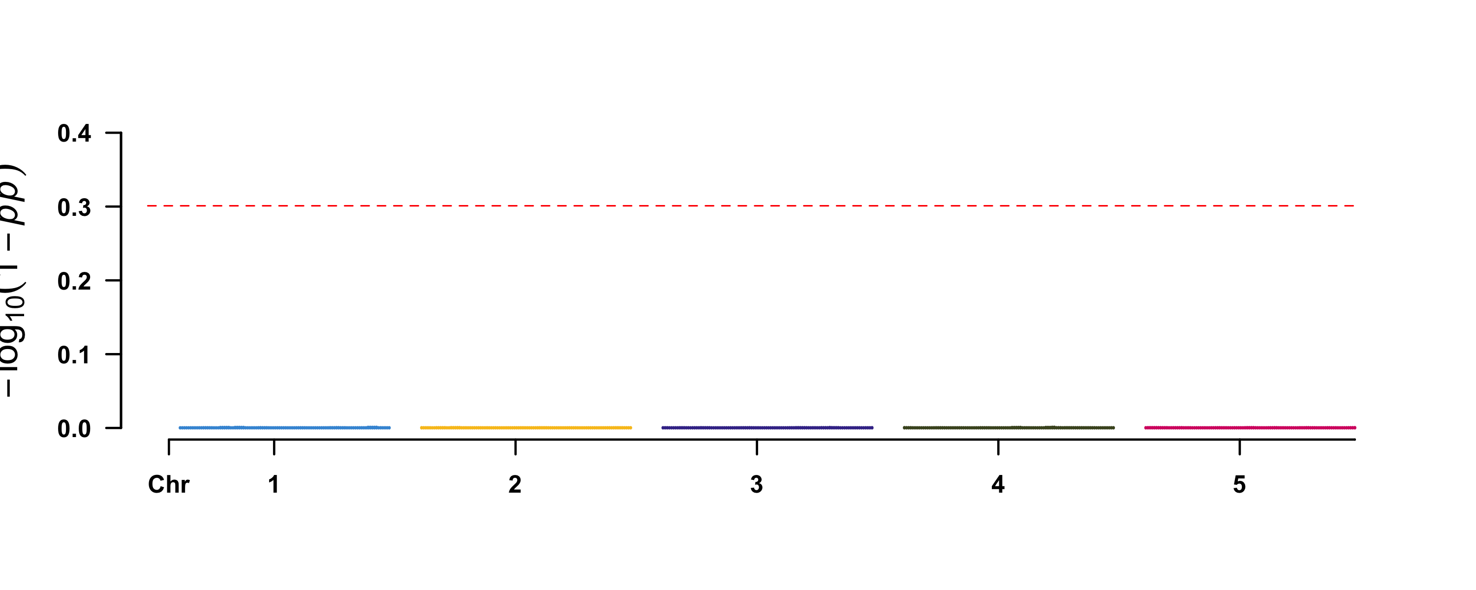
Step 5 — Manhattan plot of posterior probability
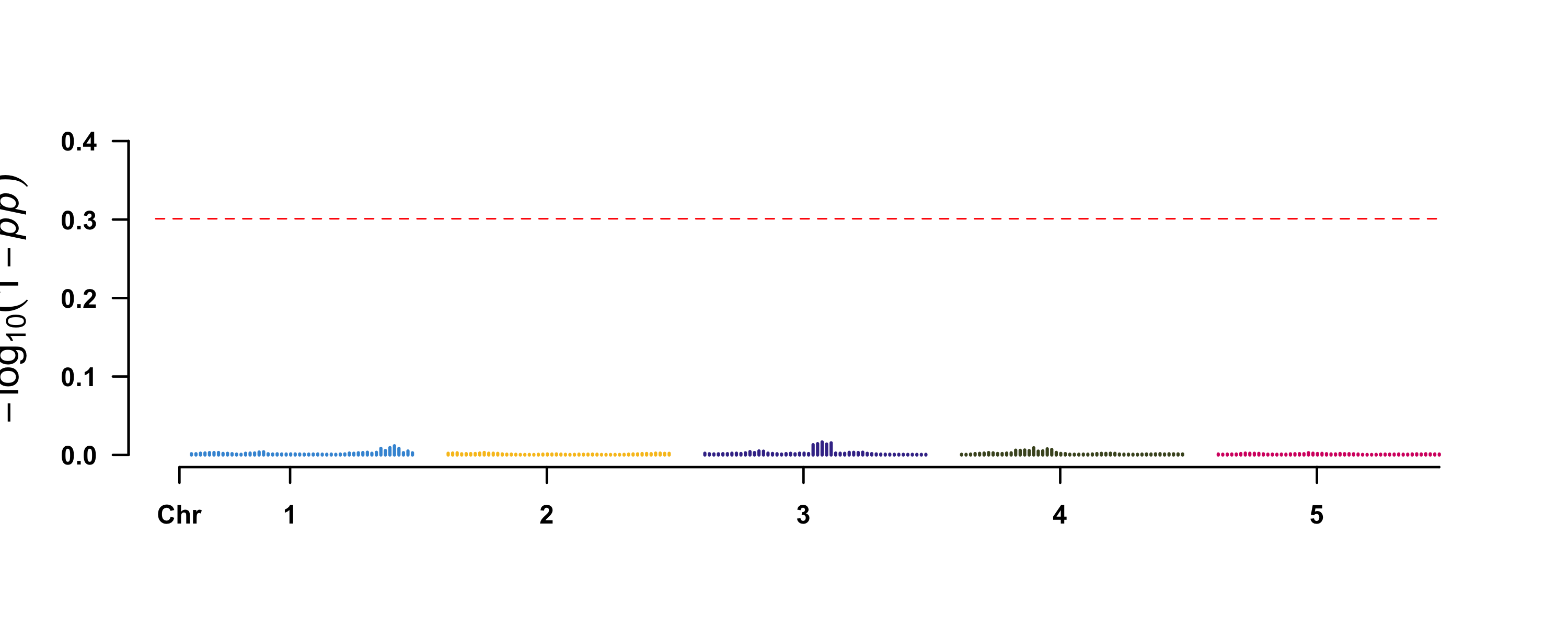
pp is smoothed and shrunk toward zero — the Manhattan of \(-\log_{10}(1 - pp)\) emphasises the markers that GWABLUP will upweight.
Code
pp_cap <- 1 - 1e-3
snp_pp_df <- data.frame(
  SNP    = map_snp$SNP,
  Chr    = map_snp$CHROM,
  Pos    = map_snp$POS,
  `1-pp` = 1 - pmin(gwas_snp$pp, pp_cap),
  check.names = FALSE
)
snp_pp_hl <- as.character(map_snp$SNP[gwas_snp$pp > 0.5])
if (length(snp_pp_hl) == 0L) snp_pp_hl <- NULL

CMplot::CMplot(
  snp_pp_df,
  type           = "h",
  plot.type      = "m",
  LOG10          = TRUE,
  threshold      = 0.5,
  threshold.lty  = 2,
  threshold.lwd  = 1,
  threshold.col  = "red",
  amplify        = FALSE,
  highlight      = snp_pp_hl,
  highlight.text = snp_pp_hl,
  highlight.col  = NULL,
  file.output    = FALSE,
  verbose        = FALSE,
  ylab           = expression(-log[10](1 - italic(pp)))
)
Step 6 — GWAS-assisted prediction (GWABLUP)
GWABLUP re-weights the genomic relationship matrix using the per-SNP pp values from the GWAS scan. Markers with high pp get heavier weights; the resulting weighted GRM enters a second mixed-model fit.
Code
fit_snp_wa <- gwablup(
  y           = y_snp,
  markers     = list(snp_add = W_snp),
  gwas_result = gwas_snp,
  ref_markers = list(snp_add = W_snp),
  trait       = "continuous"
)

kable(data.frame(
  model = c("GBLUP", "GWABLUP"),
  h2    = c(as.numeric(fit_snp_g$varcomp$h2["snp_add"]),
            as.numeric(fit_snp_wa$varcomp$h2["snp_add"]))
), digits = 4,
caption = "SNP architecture — h² captured by GBLUP vs GWABLUP")| model | h2 |
|---|---|
| GBLUP | 0.3669 |
| GWABLUP | 0.4320 |
Graceful degradation. When the training-set GWAS is underpowered, the pp values are near-uniform and the re-weighted GRM is numerically close to the baseline GBLUP G. gwablup() then collapses to GBLUP — it does not hurt accuracy in underpowered regimes, it just stops helping.
Microhaplotype-based GWAS
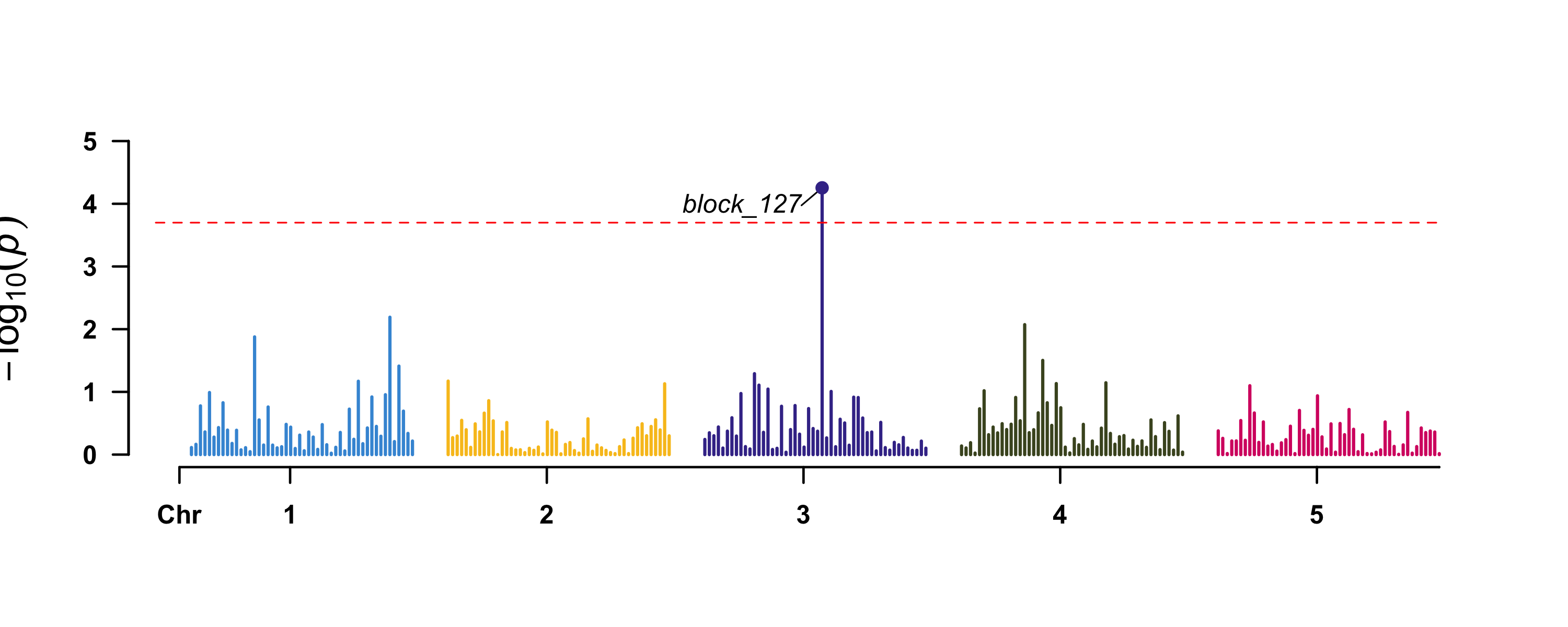
The same flow applies with markers = list(mh_add = d$mh). Each microhaplotype block produces one statistic per block (not per allele); the Manhattan x-axis uses physical positions from d$map_mh.
Code
y_mh <- setNames(d$pheno$y_cont_qtl_mh, ids)
mh   <- d$mh
rownames(mh) <- ids

fit_mh_g <- masreml(
  y       = y_mh,
  markers = list(mh_add = mh),
  method  = "auto",
  trait   = "continuous",
  verbose = FALSE
)

gwas_mh <- run_gwas(
  markers     = list(mh_add = mh),
  y           = y_mh,
  masreml_fit = fit_mh_g,
  ref_markers = list(mh_add = mh)
)
Code
top10_mh_idx <- order(-gwas_mh$pp)[seq_len(10L)]
kable(data.frame(
  Block = map_mh$block_id[top10_mh_idx],
  CHR   = map_mh$chr[top10_mh_idx],
  POS   = mh_pos[top10_mh_idx],
  pval  = signif(gwas_mh$pval[top10_mh_idx], 3),
  pp    = round(gwas_mh$pp[top10_mh_idx], 3)
), caption = "Top 10 microhaplotype blocks ranked by posterior probability")| Block | CHR | POS | pval | pp |
|---|---|---|---|---|
| block_127 | 3 | 6250000 | 5.57e-05 | 0.038 |
| block_129 | 3 | 6650000 | 9.84e-02 | 0.035 |
| block_126 | 3 | 6050000 | 4.24e-01 | 0.033 |
| block_128 | 3 | 6450000 | 5.42e-01 | 0.031 |
| block_125 | 3 | 5850000 | 3.84e-01 | 0.030 |
| block_46 | 1 | 10050000 | 6.20e-01 | 0.027 |
| block_45 | 1 | 9850000 | 6.45e-03 | 0.021 |
| block_167 | 4 | 4250000 | 4.01e-01 | 0.021 |
| block_43 | 1 | 9450000 | 5.10e-01 | 0.019 |
| block_47 | 1 | 10250000 | 3.88e-02 | 0.019 |
Code
thr_mh_p <- 0.05 / n_blocks
mh_pval_df <- data.frame(
  Block = map_mh$block_id,
  Chr   = map_mh$chr,
  Pos   = mh_pos,
  pval  = pmax(gwas_mh$pval, pval_cap),
  check.names = FALSE
)
mh_pval_hl <- as.character(map_mh$block_id[gwas_mh$pval < thr_mh_p])
if (length(mh_pval_hl) == 0L) mh_pval_hl <- NULL

CMplot::CMplot(
  mh_pval_df,
  type           = "h",
  plot.type      = "m",
  LOG10          = TRUE,
  threshold      = thr_mh_p,
  threshold.lty  = 2,
  threshold.col  = "red",
  amplify        = FALSE,
  highlight      = mh_pval_hl,
  highlight.text = mh_pval_hl,
  highlight.col  = NULL,
  file.output    = FALSE,
  verbose        = FALSE,
  ylab           = expression(-log[10](italic(p)))
)
Code
mh_pp_df <- data.frame(
  Block  = map_mh$block_id,
  Chr    = map_mh$chr,
  Pos    = mh_pos,
  `1-pp` = 1 - pmin(gwas_mh$pp, pp_cap),
  check.names = FALSE
)
mh_pp_hl <- as.character(map_mh$block_id[gwas_mh$pp > 0.5])
if (length(mh_pp_hl) == 0L) mh_pp_hl <- NULL

CMplot::CMplot(
  mh_pp_df,
  type           = "h",
  plot.type      = "m",
  LOG10          = TRUE,
  threshold      = 0.5,
  threshold.lty  = 2,
  threshold.col  = "red",
  amplify        = FALSE,
  highlight      = mh_pp_hl,
  highlight.text = mh_pp_hl,
  highlight.col  = NULL,
  file.output    = FALSE,
  verbose        = FALSE,
  ylab           = expression(-log[10](1 - italic(pp)))
)
GWABLUP on multi-allelic blocks:
Code
fit_mh_wa <- gwablup(
  y           = y_mh,
  markers     = list(mh_add = mh),
  gwas_result = gwas_mh,
  ref_markers = list(mh_add = mh),
  trait       = "continuous"
)

kable(data.frame(
  model = c("Microhaplotype-GBLUP", "Microhaplotype-GWABLUP"),
  h2    = c(as.numeric(fit_mh_g$varcomp$h2["mh_add"]),
            as.numeric(fit_mh_wa$varcomp$h2["mh_add"]))
), digits = 4,
caption = "Microhaplotype architecture — h² captured by GBLUP vs GWABLUP")| model | h2 |
|---|---|
| Microhaplotype-GBLUP | 0.3328 |
| Microhaplotype-GWABLUP | 0.2343 |
QTL recovery sanity check
Because the demo data ships with the true QTL positions in d$qtl$snp_idx and d$qtl$mh_idx, we can verify that the GWAS scan recovers them — the median pp at QTL markers should be substantially higher than at non-QTL markers.
Code
# Map allele-level QTL indices to block ids for the MH path
qtl_block_names <- unique(d$allele_freq$haplotype[d$qtl$mh_idx])
qtl_blocks      <- as.integer(sub("block_", "", qtl_block_names))

kable(data.frame(
  path        = c("SNP", "Microhaplotype"),
  pp_at_QTL   = c(median(gwas_snp$pp[d$qtl$snp_idx]),
                  median(gwas_mh$pp[qtl_blocks])),
  pp_non_QTL  = c(median(gwas_snp$pp[-d$qtl$snp_idx]),
                  median(gwas_mh$pp[-qtl_blocks]))
), digits = 3,
caption = "Median posterior probability at true QTL vs non-QTL markers")| path | pp_at_QTL | pp_non_QTL |
|---|---|---|
| SNP | 0.001 | 0.001 |
| Microhaplotype | 0.005 | 0.003 |
The ratio between the two columns is a discrimination diagnostic — a ratio of ~2× or better indicates the GWAS resolves the QTL signal above background noise on this demo. On real data, expect a similar or stronger separation when the trait is well powered and the marker density is appropriate.
Working with the GWAS output
Code
# Markers passing a Bonferroni threshold
bonferroni <- 0.05 / n_snp
sum(gwas_snp$pval < bonferroni)
[1] 0Code
# Markers passing a posterior-probability threshold
sum(gwas_snp$pp > 0.5)
[1] 0run_gwas() does not apply multiple-testing correction itself — the choice (Bonferroni / FDR / posterior threshold) is left to the analyst, since the appropriate method depends on whether you want a strict family-wise error guarantee, an expected-FDR control, or a Bayesian posterior threshold.
See also
-
run_gwas()·gwablup() - Theory overview — Meuwissen 2024 framework
- GWAS with masbayes — BayesR PIP-based alternative
-
masreml/examples/04_gwas.R— full source for this tutorial