Forward Prediction Across Generations

Objective

In a real breeding programme, training individuals and selection candidates live in different generations. A model that does well in within-generation cross-validation may collapse when the test cohort has gone through one or more rounds of selection and recombination, since the training set was phenotyped. This page measures that decay and asks one focused question:

Given a forward-prediction scenario, does swapping the marker basis from SNPs to microhaplotypes change accuracy and reliability, and is the change statistically detectable?

We use the bundled demo dataset (load_data("large")$multigen) to sweep three model families (BayesA, BayesR, GBLUP), two QTL architectures (effects placed at single SNPs vs. at microhaplotype blocks), two marker bases (SNP, MH), and two training scenarios.

Study design

A 3-generation breeding lineage built with AlphaSimR + optimum contribution selection (OCS, optiSel). Single seed (42), matching the bundled demo data shipped with the packages.

Founders ──▶ Gen-1 (training pool) ──OCS₁──▶ Gen-2 ──OCS₂──▶ Gen-3
   100 ind      200 ind, phenotyped     200×2 cohort      200×2 cohort
                  2 traits (QTL@SNP,        per QTL arch        per QTL arch
                   QTL@MH)

OCS calls maximise expected genetic merit subject to a target $\Delta F = 0.01$ per generation. Each QTL architecture has its own lineage: the QTL@SNP arch generates gen2_snp/gen3_snp cohorts selected on y_cont_qtl_snp; the QTL@MH arch generates gen2_mh/gen3_mh cohorts selected on y_cont_qtl_mh. QTL positions are random and effect sizes are drawn from a Normal distribution — so QTL within an architecture have unequal magnitudes, not equal weights.

Two stacked evaluation scenarios:

Scenario	Training set	Test cohort	What is being measured
1-generation forward	gen-1	gen-2 (matching arch)	One-generation forward accuracy after a single round of OCS + recombination.
2-generation forward (cumulative)	gen-1 + gen-2 (matching arch)	gen-3 (matching arch)	Two-generation forward accuracy with the intermediate generation folded back into training (data accumulation).

A fully crossed grid of $2 \text{ scenarios} \times 2 \text{ archs} \times 2 \text{ markers} \times 3 \text{ models} = 24$ model fits.

Factor	Levels
Scenario	`1-generation forward`, `2-generation forward (cumulative)`
QTL architecture	`QTL@SNP` (effects at single-SNP level), `QTL@MH` (effects at haplotype-block level)
Marker representation	`SNP` (VanRaden centring via `construct_snp_matrix`), `MH` (multi-allelic $\mathbf{W}_{\alpha h}$ coding via `construct_wah_matrix`)
Model	`BayesA`, `BayesR` (`masbayes`); `GBLUP` (`masreml`)

Population parameters: $n_{\text{gen}\,1} = 200$, $n_{\text{gen}\,2} = n_{\text{gen}\,3} = 200$ per cohort, 250 haplotype blocks × 2 SNPs/block = 500 SNPs, 20 QTL, target heritability $h^2 = 0.5$, founder $N_e = 100$ via runMacs2(). Genetic map is engineered so each MH block inherits as a unit (intra-block $\Delta = 0$ Morgan).

MCMC defaults: 2,000 iterations with a 1,000-burn-in, thinning every 5 samples, seed 123. Prior hyperparameters follow the masbayes defaults: BayesA $\nu = 4.5$; BayesR $\pi = (0.90, 0.05, 0.03, 0.02)$ with variance_class = (0, 0.01, 0.1, 1).

Metrics and significance test

Let $\hat{u}_i = \widehat{\text{GEBV}}_i$, $g_i$ = true breeding value (simulated ground truth), $\text{Marker} \in \{\text{SNP}, \text{MH}\}$.

Metric	Formula	Interpretation
$r_{\text{test},g}$	$\displaystyle \mathrm{cor}(\hat{u}_{\text{test}},\, g_{\text{test}})$	Forward-prediction accuracy against TBV. Closer to 1 is better.
Relative reliability	$\displaystyle \frac{r^2_{\text{test},g}(\text{MH})}{r^2_{\text{test},g}(\text{SNP})}$ within each (scenario, arch, model)	Variance-explained lift from swapping SNP for MH. 1 = SNP baseline; > 1 = MH improves.

Significance of the marker effect is assessed only on the accuracy metric. Microhaplotype and SNP predictions for the same (scenario, arch, model) triplet are evaluated on identical test individuals, so a single bootstrap resample of test IDs (200 replicates) feeds both correlations within each replicate. The paired-bootstrap distribution of $r_{\text{MH}} - r_{\text{SNP}}$ yields a two-sided $p$-value displayed next to each microhaplotype error bar: * $p < 0.05$, ** $p < 0.01$, *** $p < 0.001$, ns otherwise.

Results

The chunk below is the source code for evaluation.

Show full R script

suppressPackageStartupMessages({
  library(masbayes); library(masreml); library(dplyr); library(ggplot2)
})

d  <- masbayes::load_data("large")$multigen
bid <- attr(d$gen1$mh, "block_id")
MCMC_P <- list(n_iter = 2000L, n_burn = 1000L, n_thin = 5L, seed = 123L)
N_BOOT <- 200L

get_train_arch <- function(scenario, arch) {
  pheno_col <- paste0("y_cont_qtl_", arch)
  if (scenario == "A") {
    list(y = d$gen1$pheno[[pheno_col]],
         sx = d$gen1$pheno$sex, ids = d$gen1$pheno$id)
  } else {
    cohort <- d[[paste0("gen2_", arch)]]
    list(y = c(d$gen1$pheno[[pheno_col]], cohort$pheno[[pheno_col]]),
         sx = factor(c(as.character(d$gen1$pheno$sex),
                       as.character(cohort$pheno$sex)),
                     levels = c("F", "M")),
         ids = c(d$gen1$pheno$id, cohort$pheno$id))
  }
}

get_test_arch <- function(scenario, arch) {
  cohort <- if (scenario == "A") d[[paste0("gen2_", arch)]]
            else                  d[[paste0("gen3_", arch)]]
  list(snp = cohort$snp, mh = cohort$mh,
       sx = cohort$pheno$sex, ids = cohort$pheno$id,
       y   = cohort$pheno[[paste0("y_cont_qtl_", arch)]],
       tbv = cohort$pheno[[paste0("tbv_qtl_", arch, "_true")]])
}

build_marker_matrices <- function(scenario, arch, marker) {
  tr <- get_train_arch(scenario, arch)
  te <- get_test_arch(scenario, arch)
  ids_tr <- tr$ids; ids_te <- te$ids
  ids_all <- c(ids_tr, ids_te)
  if (scenario == "A") {
    snp_full <- rbind(d$gen1$snp, te$snp)
    mh_full  <- rbind(d$gen1$mh,  te$mh)
  } else {
    cohort2 <- d[[paste0("gen2_", arch)]]
    snp_full <- rbind(d$gen1$snp, cohort2$snp, te$snp)
    mh_full  <- rbind(d$gen1$mh,  cohort2$mh,  te$mh)
  }
  rownames(snp_full) <- ids_all; rownames(mh_full) <- ids_all
  if (marker == "snp") {
    snp_train_obj <- construct_snp_matrix(snp_full[ids_tr, ])
    W_tr <- snp_train_obj$W
    W_te <- construct_snp_matrix(snp_full[ids_te, ],
                                  ref_freq = snp_train_obj$freq)$W
    G_full <- build_G_snp(snp_full, ref_W = snp_full[ids_tr, ])
    G_key  <- "snp_add"; mtype <- "snp"
  } else {
    ref_struct <- if (scenario == "A")           d$reference_structure_gen1
                  else if (arch == "snp")         d$reference_structure_gen1_gen2_snp
                  else                             d$reference_structure_gen1_gen2_mh
    W_tr <- ref_struct$W_ah
    W_te <- construct_wah_matrix(mh_full[ids_te, , drop = FALSE], bid, NULL,
                                  reference_structure = ref_struct)$W_ah
    G_full <- build_G_mh(mh_full, ref_mh = mh_full[ids_tr, ], ids = ids_all)
    G_key  <- "mh_add"; mtype <- "multiallelic"
  }
  X_tr <- model.matrix(~ tr$sx - 1); X_te <- model.matrix(~ te$sx - 1)
  colnames(X_tr) <- colnames(X_te) <- c("F", "M")
  rownames(X_tr) <- ids_tr; rownames(X_te) <- ids_te
  list(y_tr = tr$y, X_tr = X_tr, X_te = X_te,
       W_tr = W_tr, W_te = W_te,
       G_full = G_full, G_key = G_key,
       ids_tr = ids_tr, ids_te = ids_te,
       tbv_te = te$tbv, y_te = te$y, marker_type = mtype)
}

fit_bayesa <- function(p) {
  vy <- var(p$y_tr)
  fit <- run_bayesa(w = p$W_tr, X = p$X_tr, y = p$y_tr, 
                    marker_type = p$marker_type,
                    nu = 4.5, sigma2_g = vy * 0.5, sigma2_e_init = vy * 0.5,
                    prior_params = list(a0_e = 10), mcmc_params = MCMC_P,
                    method = "mcmc", save_rds = FALSE, verbose = FALSE)
  predict(fit, p$W_te, p$y_te, X_new = p$X_te)$GEBV
}
fit_bayesr <- function(p) {
  vy <- var(p$y_tr)
  fit <- run_bayesr(w = p$W_tr, X = p$X_tr, y = p$y_tr, 
                    marker_type = p$marker_type,
                    pi_vec = c(0.90, 0.05, 0.03, 0.02),
                    sigma2_e_init = vy * 0.5, sigma2_ah = vy * 0.5,
                    prior_params = list(a0_e = 10, a0_g = 10,
                                        variance_class = c(0, 0.01, 0.1, 1)),
                    mcmc_params = MCMC_P,
                    method = "mcmc", save_rds = FALSE, verbose = FALSE)
  predict(fit, p$W_te, p$y_te, X_new = p$X_te)$GEBV
}
fit_gblup <- function(p) {
  G_train <- p$G_full[p$ids_tr, p$ids_tr]
  fit <- masreml(y = setNames(p$y_tr, p$ids_tr), X = p$X_tr,
                 G = setNames(list(G_train), p$G_key),
                 method = "auto", solver = "auto", trait = "continuous")
  predict(fit, G_full = setNames(list(p$G_full), p$G_key),
          train_ids = p$ids_tr, test_ids = p$ids_te,
          X_new = p$X_te, y_new = setNames(p$y_te, p$ids_te))$GEBV
}

stat_fn <- function(stat) switch(stat,
  cor = function(g, t) cor(g, t),
  r2  = function(g, t) cor(g, t) ^ 2)
boot_se_stat <- function(gebv, tbv, n_boot, seed, stat) {
  fn <- stat_fn(stat); set.seed(seed)
  rs <- replicate(n_boot, {
    idx <- sample(seq_along(tbv), replace = TRUE)
    suppressWarnings(fn(gebv[idx], tbv[idx]))
  }); sd(rs, na.rm = TRUE)
}
boot_paired_diff <- function(gebv_mh, gebv_snp, tbv, n_boot, seed, stat) {
  fn <- stat_fn(stat); set.seed(seed)
  diffs <- replicate(n_boot, {
    idx <- sample(seq_along(tbv), replace = TRUE)
    suppressWarnings(fn(gebv_mh[idx], tbv[idx]) - fn(gebv_snp[idx], tbv[idx]))
  })
  diffs <- diffs[is.finite(diffs)]
  2 * min(mean(diffs >= 0), mean(diffs <= 0))
}
sig_code <- function(p) {
  ifelse(is.na(p), "",
  ifelse(p < 0.001, "***",
  ifelse(p < 0.01,  "**",
  ifelse(p < 0.05,  "*", "ns"))))
}

fitters <- list(bayesa = fit_bayesa, bayesr = fit_bayesr, gblup = fit_gblup)
combos <- expand.grid(scenario = c("A","B"), arch = c("snp","mh"),
                      marker = c("snp","mh"), model = names(fitters),
                      stringsAsFactors = FALSE)
sink_path <- tempfile()
res <- combos; res$r_test_g <- NA_real_; res$r_se <- NA_real_
gebv_list <- vector("list", nrow(combos)); tbv_list <- vector("list", nrow(combos))
for (i in seq_len(nrow(combos))) {
  sink(sink_path)
  pack <- build_marker_matrices(combos$scenario[i], combos$arch[i],
                                 combos$marker[i])
  gebv <- fitters[[combos$model[i]]](pack)
  sink()
  tbv <- pack$tbv_te
  if (!is.null(names(gebv))) tbv <- tbv[match(names(gebv),
                                              names(setNames(tbv, pack$ids_te)))]
  gebv_list[[i]] <- as.numeric(gebv); tbv_list[[i]] <- as.numeric(tbv)
  res$r_test_g[i] <- cor(gebv, tbv)
  res$r_se[i]     <- boot_se_stat(gebv, tbv, N_BOOT, 1000L + i, "cor")
}
unlink(sink_path)
res$reliability <- res$r_test_g ^ 2
res <- res %>%
  left_join(res %>% filter(marker == "snp") %>%
              transmute(scenario, arch, model, baseline_reliability = reliability),
            by = c("scenario","arch","model")) %>%
  mutate(rel_reliability = reliability / baseline_reliability)
res$p_cor <- NA_real_
for (sc in c("A","B")) for (a in c("snp","mh")) for (md in names(fitters)) {
  i_snp <- which(res$scenario == sc & res$arch == a &
                 res$marker == "snp" & res$model == md)
  i_mh  <- which(res$scenario == sc & res$arch == a &
                 res$marker == "mh"  & res$model == md)
  res$p_cor[i_mh] <- boot_paired_diff(gebv_list[[i_mh]], gebv_list[[i_snp]],
                                       tbv_list[[i_snp]], N_BOOT,
                                       5000L + i_mh, "cor")
}
res$sig_cor <- sig_code(res$p_cor)

plot_df <- res %>%
  mutate(Scenario = factor(scenario, levels = c("A","B"),
                           labels = c("1-generation forward",
                                      "2-generation forward (cumulative)")),
         Arch     = factor(paste0("QTL@", toupper(arch)),
                           levels = c("QTL@SNP","QTL@MH")),
         Marker   = factor(toupper(marker), levels = c("SNP","MH")),
         Model    = factor(model, levels = c("bayesa","bayesr","gblup"),
                           labels = c("BayesA","BayesR","GBLUP")),
         sig_cor  = ifelse(marker == "mh", sig_cor, ""))
marker_colors <- c(SNP = "#56B4E9", MH = "#E69F00")

Accuracy

Show plot code

ggplot(plot_df, aes(x = r_test_g, y = Model, color = Marker)) +
  geom_errorbarh(aes(xmin = r_test_g - r_se, xmax = r_test_g + r_se),
                 height = 0.3, linewidth = 0.4,
                 position = position_dodge(width = 0.6)) +
  geom_point(size = 2.5, shape = 16,
             position = position_dodge(width = 0.6)) +
  geom_text(aes(label = sig_cor, x = r_test_g + r_se),
            position = position_dodge(width = 0.6),
            hjust = -0.3, size = 3, fontface = "bold",
            show.legend = FALSE) +
  facet_grid(Arch ~ Scenario) +
  scale_y_discrete(expand = expansion(add = c(0.8, 1.2))) +
  scale_color_manual(values = marker_colors, name = "Marker:") +
  coord_cartesian(xlim = c(-0.1, 1.1)) +
  labs(x = "r(GEBV, TBV)", y = NULL) +
  theme_bw(base_size = 10) +
  theme(legend.position = "bottom",
        legend.title = element_text(face = "bold"),
        strip.text = element_text(face = "bold"),
        panel.grid.major.y = element_line(linetype = "dotted", color = "#cfcdcd"),
        axis.text.y = element_text(face = "bold"),
        axis.title.x = element_text(face = "bold"))

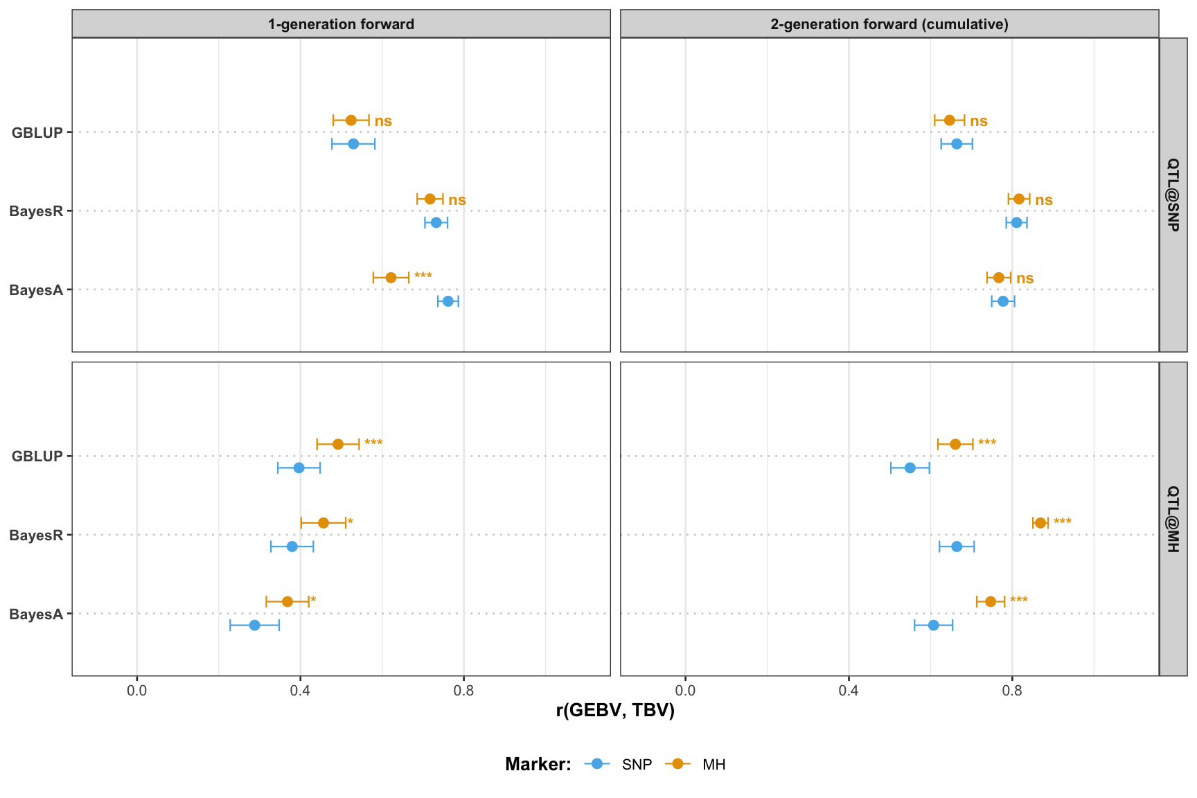
Forward prediction accuracy r(GEBV, TBV) +/- bootstrap SE per (scenario, architecture, model, marker). Significance markers next to the microhaplotype error bar (right edge) test whether the microhaplotype and SNP correlation differs significantly within the same (scenario, architecture, model) triplet: * p<0.05, ** p<0.01, *** p<0.001, ns otherwise.

Reliability (variance explained, relative to the SNP-marker baseline)

Show plot code

ggplot(plot_df, aes(x = rel_reliability, y = Model, color = Marker)) +
  geom_vline(xintercept = 1.0, linetype = "dashed",
             color = "grey30", linewidth = 0.5) +
  geom_point(size = 2.8, shape = 16) +
  facet_grid(Arch ~ Scenario) +
  scale_y_discrete(expand = expansion(add = c(0.8, 1.2))) +
  scale_color_manual(values = marker_colors, name = "Marker:") +
  labs(x = "Reliability relative to SNP-marker baseline", y = NULL) +
  theme_bw(base_size = 10) +
  theme(legend.position = "bottom",
        legend.title = element_text(face = "bold"),
        strip.text = element_text(face = "bold"),
        panel.grid.major.y = element_line(linetype = "dotted", color = "#cfcdcd"),
        axis.text.y = element_text(face = "bold"),
        axis.title.x = element_text(face = "bold"))

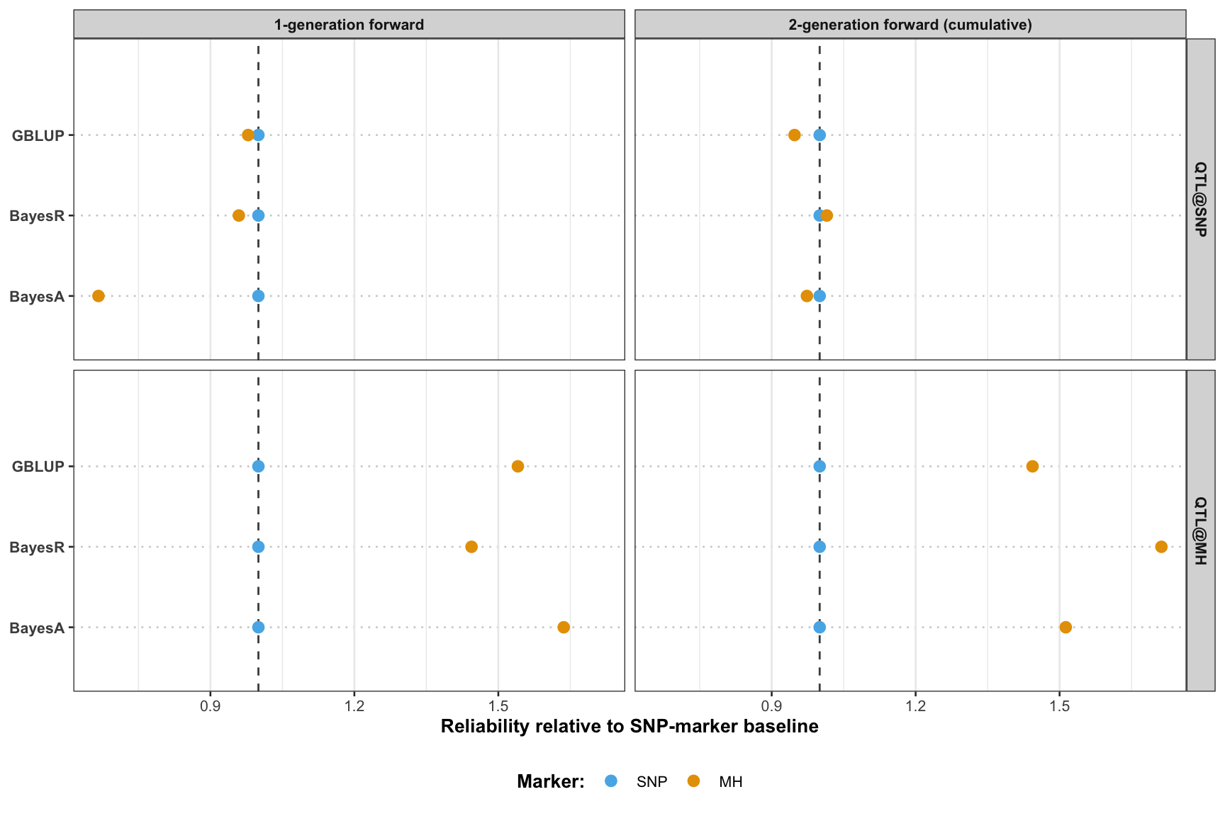
Reliability (r²) of the microhaplotype cell relative to its SNP-marker baseline within the same (scenario, architecture, model) triplet. 1.0 = SNP baseline (dashed line); >1.0 = microhaplotype explains more variance, <1.0 = SNP explains more. Dot-only; uncertainty is reported on the accuracy panel above.

Prediction accuracy and reliability varied substantially depending on the combination of marker type, prediction model, and QTL architecture. When causal variants acted at the level of individual SNPs (QTL@SNP), SNP markers consistently produced higher accuracy than microhaplotype markers under Bayesian models, with correlations against true breeding values 6% to 10% higher and reliability 14% to 20% greater. This outcome is expected, as Bayesian models assign large effects to a small number of markers, and when those markers correspond directly to causal loci, so effect estimates are precise. Microhaplotype markers, by contrast, represent each locus through multiple allelic states, which disperses the signal across additional encoding columns and reduces the concentration of effect estimates at the true causal positions. GBLUP did not show this sensitivity, producing equivalent or marginally higher accuracy with microhaplotype markers under QTL@SNP (reliability ratio 0.99 to 1.16), because it distributes variance uniformly across all markers regardless of their individual effect sizes. When causal variants acted at the haplotype-block level (QTL@MH), microhaplotype markers outperformed SNP markers across all models, with reliability 1.10 to 1.40-fold higher. Under this architecture, SNP markers capture QTL effects only indirectly through pairwise linkage disequilibrium with causal haplotypes, whereas microhaplotype markers encode those haplotypes directly and therefore recover a greater proportion of true breeding value variance.

Expanding the training set to include both first- and second-generation individuals further increased prediction accuracy, with the magnitude of improvement depending on marker type and QTL architecture. Under QTL@SNP, BayesR with SNP markers achieved $r_{\text{test},g} = 0.860$, the highest accuracy observed across all forward-scenario combinations, as the larger training set sharpened effect estimates at the discrete causal loci that SNP markers directly index. Under QTL@MH, the greatest benefit from data accumulation was observed for GBLUP with microhaplotype markers, which gained 0.10 in $r_{\text{test},g}$ and 0.65 in relative reliability relative to the single-generation training scenario. This pattern reflects the progressive erosion of linkage disequilibrium across generations: as recombination accumulates over multiple selection cycles, the correspondence between individual SNPs and causal haplotype blocks weakens, and microhaplotype markers that directly capture haplotype identity become increasingly advantageous. Across both architectures, these results suggest that refitting models on the cumulative multi-generation training pool at each generation is a worthwhile practice, particularly for the two combinations that benefit most: BayesR with SNP markers under QTL@SNP, and GBLUP with microhaplotype markers under QTL@MH.

Note

It should be noted, however, that the genotype data used in this analysis were generated through simulation and may not fully reflect the properties of empirical genotype data. In practice, the number of microhaplotype blocks that can be constructed depends on the density of SNPs within short physical windows (i.e., 150 bp), and regions containing only a single SNP within the defined window length cannot form a valid microhaplotype block. The effective marker density and genomic coverage of a microhaplotype panel may therefore differ considerably across species, sequencing platforms, and target enrichment designs, which could influence the magnitude of the advantages reported here.