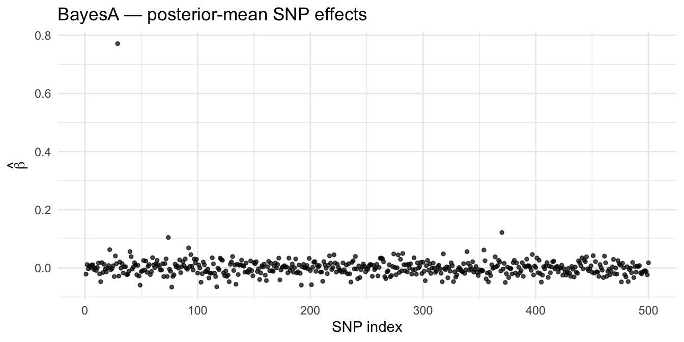
This tutorial fits Bayesian genomic prediction with masbayes: BayesA (Student-\(t\) prior, continuous shrinkage) and BayesR (4-class mixture prior, sparse selection), via both MCMC and EM, on SNP and phased microhaplotype data. Cross-validation in masbayes is manual — the package exposes single-fit functions only — so a worked-out CV loop is included.
Setup
Code
library(masbayes)library(masreml)# for evaluate_prediction() — reused on Bayesian GEBVslibrary(ggplot2)library(knitr)d<-load_data("large")y<-setNames(d$pheno$y_cont_qtl_snp, d$pheno$id)X_fixed<-stats::model.matrix(~sex, data =d$pheno)# Tutorial-scale MCMC params (same as masbayes/examples/04_gwas.R).# Production runs should use n_iter = 20000, n_burn = 5000, n_thin = 5L.mcmc<-list(n_iter =2000L, n_burn =1000L, n_thin =5L, seed =42L)
Note
Production MCMC. The chunks below use n_iter = 2000 for fast tutorial rendering. For published analyses on real-data scale, use n_iter = 20000, n_burn = 5000, n_thin = 5L (or longer) and inspect trace plots before trusting posterior summaries.
SNP workflow
Build the design matrix W
The Bayesian fitters take a pre-standardised design matrix \(\mathbf{W}\); the per-column sum-of-squares \(\mathbf{w}'\mathbf{w}\) is computed internally, so you no longer pass it. construct_snp_matrix() returns a list — extract $W.
List of 4
 $ W   : num [1:200, 1:500] 0.22 0.22 0.22 0.22 0.22 0.22 0.22 0.22 0.22 0.22 ...
  ..- attr(*, "dimnames")=List of 2
  .. ..$ : chr [1:200] "IND001" "IND002" "IND003" "IND004" ...
  .. ..$ : chr [1:500] "SNP001" "SNP002" "SNP003" "SNP004" ...
 $ freq: Named num [1:500] 0.39 0.475 0.198 0.39 0.388 ...
  ..- attr(*, "names")= chr [1:500] "SNP001" "SNP002" "SNP003" "SNP004" ...
 $ n   : int 200
 $ p   : int 500
BayesA — full fit (MCMC)
BayesA assigns each SNP its own variance drawn from a scaled inverse-\(\chi^2\). The marginal prior on \(\beta_j\) is Student-\(t\) with heavy tails — markers in real QTL regions are allowed to keep large effects, while distant markers are shrunk hard.
Code
fit_a_mcmc<-run_bayesa( w =W_snp, y =y, X =X_fixed, marker_type ="snp", nu =4.5, sigma2_g =var(y)*0.5, sigma2_e_init =var(y)*0.5, method ="mcmc", response_type ="gaussian", mcmc_params =mcmc, verbose =FALSE)
============================================================
 masbayes — BayesA with MCMC algorithm
============================================================
 Response type   : gaussian
 Observations    : n = 200, alleles p = 500
 Runtime         : 0.68 seconds

 Heritability (h2): 0.534

 MCMC Diagnostics
 ----------------------------------------
   Parameter             ESS    Geweke Z
   sigma2_e            200.0       -1.12
   mu                    3.1       -0.61
   beta (median)       200.0       -0.09
 ----------------------------------------

 Run summary(fit) for full report.
============================================================
kable(data.frame(metric =c("Heritability (h²)","Residual variance","Genetic variance"), value =c(fit_a_mcmc$h2,fit_a_mcmc$sigma2_e,fit_a_mcmc$sigma2_g)), digits =4, caption ="BayesA — variance components and h²")
BayesA — variance components and h²
metric
value
Heritability (h²)
0.5341
Residual variance
0.8611
Genetic variance
0.9870
Predict on held-out candidates
Code
train_idx<-d$train_idxtest_idx<-d$test_idxfit_a_train<-run_bayesa( w =W_snp[train_idx, , drop =FALSE], y =y[train_idx], X =X_fixed[train_idx, , drop =FALSE], marker_type ="snp", nu =4.5, sigma2_g =var(y[train_idx])*0.5, sigma2_e_init =var(y[train_idx])*0.5, method ="mcmc", response_type ="gaussian", mcmc_params =mcmc, verbose =FALSE)
============================================================
 masbayes — BayesA with MCMC algorithm
============================================================
 Response type   : gaussian
 Observations    : n = 160, alleles p = 500
 Runtime         : 0.52 seconds

 Heritability (h2): 0.493

 MCMC Diagnostics
 ----------------------------------------
   Parameter             ESS    Geweke Z
   sigma2_e            200.0       -0.90
   mu                    3.0       -0.63
   beta (median)       200.0       -0.06
 ----------------------------------------

 Run summary(fit) for full report.
============================================================
Code
pred_a<-predict(fit_a_train, newdata =W_snp[test_idx, , drop =FALSE], X_new =X_fixed[test_idx, , drop =FALSE], y_new =y[test_idx])kable(as.data.frame(pred_a$metrics), digits =4, caption ="BayesA — held-out test accuracy")
BayesA — held-out test accuracy
R2
RMSE
accuracy
bias
0.3451
1.1687
0.5874
1.2739
BayesA — EM (MAP, faster)
For point estimates without posterior samples, switch method = "em". EM converges in tens of iterations; MCMC typically wants thousands.
Code
fit_a_em<-run_bayesa( w =W_snp, y =y, X =X_fixed, marker_type ="snp", nu =4.5, sigma2_g =var(y)*0.5, sigma2_e_init =var(y)*0.5, method ="em", response_type ="gaussian", verbose =FALSE)
============================================================
 masbayes — BayesA with EM algorithm
============================================================
 Response type   : gaussian
 Observations    : n = 200, alleles p = 500
 Runtime         : 0.02 seconds

 Heritability (h2): 0.514

 EM Convergence  : completed in fixed iterations (see fit$em_params)

 Run summary(fit) for full report.
============================================================
============================================================
 masbayes Summary — BayesA with EM
============================================================
 Model info
 ----------------------------------------
   Response type : gaussian
   Observations  : n = 200
   Alleles       : p = 500
   Fold id       : 0
   Runtime       : 0.02 seconds

 Training fit
 ----------------------------------------
   h2            : 0.5142
   sigma2_g      : 0.6797
   sigma2_e      : 0.6422
   accuracy (r)  : 0.8235
   R^2           : 0.6781
   RMSE          : 0.8014
   bias (slope)  : 1.331

 Variance components
 ----------------------------------------
   (BayesA: per-marker variances binned into tertiles)
   small    : mean=0.003893  range=[0.003846, 0.003921]  n_markers=167
   medium   : mean=0.003954  range=[0.003922, 0.003991]  n_markers=166
   large    : mean=0.005482  range=[0.003992, 0.228]  n_markers=167

 EM run — no MCMC diagnostics.

 GEBV (training) quantiles
 ----------------------------------------
   min=-1.639  Q1=-0.2604  median=0.423  Q3=0.9963  max=2.213

 beta_hat
 ----------------------------------------
   length=500  nonzero=500  mean|beta|=0.01526  max|beta|=0.881
   beta_samples : 1 x 500 (draws x alleles)
   sigma2_j_samples : 1 x 500 (draws x alleles)

 Top 10 alleles by |beta_hat|
 ----------------------------------------
 rank index        beta
    1    29  0.88100098
    2   370  0.08001892
    3    74  0.06652395
    4   339  0.05915733
    5   201 -0.05121759
    6    40  0.04720630
    7    49 -0.04633735
    8   134 -0.04627253
    9   192 -0.04479819
   10   128 -0.04339833

============================================================
EM returns the MAP \(\hat\beta\) and point estimates of variance components, but no posterior intervals. Use MCMC when you need uncertainty quantification (or PIPs, for BayesR).
BayesR — full fit (MCMC)
BayesR replaces the heavy-tailed continuous prior with a discrete 4-class mixture (zero / small / medium / large). pi_vec is the prior mixture proportions; the conventional starting point is c(0.95, 0.02, 0.02, 0.01). sigma2_ah sets the total genetic variance scale.
Code
fit_r_mcmc<-run_bayesr( w =W_snp, y =y, X =X_fixed, marker_type ="snp", pi_vec =c(0.95, 0.02, 0.02, 0.01), sigma2_ah =var(y)*0.5, sigma2_e_init =var(y)*0.5, method ="mcmc", response_type ="gaussian", mcmc_params =mcmc, verbose =FALSE)
============================================================
 masbayes — BayesR with MCMC algorithm
============================================================
 Response type   : gaussian
 Observations    : n = 200, alleles p = 500
 Runtime         : 0.65 seconds

 Heritability (h2): 0.405

 MCMC Diagnostics
 ----------------------------------------
   Parameter             ESS    Geweke Z
   sigma2_e             20.5       -0.15
   mu                    4.5       -3.12
   beta (median)       200.0        0.01
 ----------------------------------------

 Run summary(fit) for full report.
============================================================
============================================================
 masbayes Summary — BayesR with MCMC
============================================================
 Model info
 ----------------------------------------
   Response type : gaussian
   Observations  : n = 200
   Alleles       : p = 500
   Fold id       : 0
   Runtime       : 0.65 seconds

 Training fit
 ----------------------------------------
   h2            : 0.4050
   sigma2_g      : 0.7082
   sigma2_e      : 1.0402
   accuracy (r)  : 0.8063
   R^2           :  0.65
   RMSE          : 0.8712
   bias (slope)  :  1.54

 Variance components
 ----------------------------------------
   zero     :                                    pi=0.2862
   small    : mean=0.0002643  95% CI=[4.257e-05, 0.001589]   pi=0.1629
   medium   : mean=0.002643  95% CI=[0.0004257, 0.01589]   pi=0.2863
   large    : mean=0.02643  95% CI=[0.004257, 0.1589]   pi=0.2645

 MCMC diagnostics (ESS / Geweke Z)
 ----------------------------------------
   sigma2_e           ESS=    20.5   Z=  -0.146
   mu                 ESS=   4.538   Z=  -3.118
   beta               ESS[min/med/max]=2.862/  200/795.6   |Z|max=4.071
   sigma2_small       ESS=   6.503   Z= -0.8128
   sigma2_medium      ESS=   6.503   Z= -0.8128
   sigma2_large       ESS=   6.503   Z= -0.8128
   pi                 ESS[min/med/max]=4.675/5.965/7.532   |Z|max=0.7672

 GEBV (training) quantiles
 ----------------------------------------
   min=-1.31  Q1=-0.09057  median=0.4095  Q3=0.8514  max=1.998

 beta_hat
 ----------------------------------------
   length=500  nonzero=500  mean|beta|=0.01257  max|beta|=0.336
   beta_samples : 200 x 500 (draws x alleles)

 Top 10 alleles by |beta_hat|
 ----------------------------------------
 rank index        beta
    1    29  0.33595895
    2   370  0.12366678
    3    74  0.07776477
    4    22  0.06313945
    5   339  0.06130299
    6   354  0.05779764
    7   201 -0.05618347
    8   451  0.05493107
    9   117 -0.04944762
   10   282  0.04791903

============================================================
The posterior of \(\pi\) tells you how concentrated the trait architecture is — a high \(\hat\pi_0\) (fraction in the zero class) indicates a sparse architecture; a low \(\hat\pi_0\) a polygenic one:
For per-marker GWAS-style output (PIPs and WPPA windows), pass map and one of windsize / windnum — see the GWAS with masbayes page.
BayesR — EM
Code
fit_r_em<-run_bayesr( w =W_snp, y =y, X =X_fixed, marker_type ="snp", pi_vec =c(0.95, 0.02, 0.02, 0.01), sigma2_ah =var(y)*0.5, sigma2_e_init =var(y)*0.5, method ="em", response_type ="gaussian", verbose =FALSE)
============================================================
 masbayes — BayesR with EM algorithm
============================================================
 Response type   : gaussian
 Observations    : n = 200, alleles p = 500
 Runtime         : 0.03 seconds

 Heritability (h2): 0.414

 EM Convergence  : completed in fixed iterations (see fit$em_params)

 Run summary(fit) for full report.
============================================================
============================================================
 masbayes Summary — BayesR with EM
============================================================
 Model info
 ----------------------------------------
   Response type : gaussian
   Observations  : n = 200
   Alleles       : p = 500
   Fold id       : 0
   Runtime       : 0.03 seconds

 Training fit
 ----------------------------------------
   h2            : 0.4143
   sigma2_g      : 0.6783
   sigma2_e      : 0.9588
   accuracy (r)  : 0.6787
   R^2           : 0.4606
   RMSE          : 0.9792
   bias (slope)  : 1.098

 Variance components
 ----------------------------------------
   zero     :                                    pi=0.9468
   small    : mean=9.516e-06  95% CI=[NA, NA]   pi=0.01997
   medium   : mean=9.449e-05  95% CI=[NA, NA]   pi=0.02034
   large    : mean=0.2646  95% CI=[NA, NA]   pi=0.01288

 EM run — no MCMC diagnostics.

 GEBV (training) quantiles
 ----------------------------------------
   min=-1.575  Q1=-0.1659  median=0.4345  Q3=0.9745  max=2.094

 beta_hat
 ----------------------------------------
   length=500  nonzero=500  mean|beta|=0.005326  max|beta|=0.9292
   beta_samples : 1 x 500 (draws x alleles)

 Top 10 alleles by |beta_hat|
 ----------------------------------------
 rank index         beta
    1    29  0.929194515
    2   370  0.567812832
    3   201 -0.410349707
    4    77 -0.344670673
    5    74  0.080019085
    6    22  0.026235356
    7   354  0.024858231
    8    92  0.017280958
    9   282  0.015901816
   10   339  0.007803829

============================================================
EM-BayesR returns hard class assignments and a MAP \(\hat\beta\). It is the right choice for very large \(p\) where MCMC mixing is the bottleneck, but loses PIP and posterior intervals.
Cross-validation (manual loop)
masbayes does not provide a cv_* wrapper — write the loop explicitly. The pattern below uses BayesA but swap to run_bayesr() without changing the scaffold (add pi_vec / sigma2_ah).
Code
set.seed(42L)n<-nrow(W_snp)K<-5Lfolds<-sample(rep(seq_len(K), length.out =n))gebv_test<-rep(NA_real_, n)for(kinseq_len(K)){tr<-which(folds!=k)te<-which(folds==k)W_tr<-W_snp[tr, , drop =FALSE]fit_k<-run_bayesa( w =W_tr, y =y[tr], X =X_fixed[tr, , drop =FALSE], marker_type ="snp", nu =4.5, sigma2_g =var(y[tr])*0.5, sigma2_e_init =var(y[tr])*0.5, method ="mcmc", response_type ="gaussian", mcmc_params =list(n_iter =1000L, n_burn =500L, n_thin =5L, seed =42L+k), verbose =FALSE)pred_k<-predict(fit_k, newdata =W_snp[te, , drop =FALSE], X_new =X_fixed[te, , drop =FALSE])gebv_test[te]<-pred_k$GEBV}
============================================================
 masbayes — BayesA with MCMC algorithm
============================================================
 Response type   : gaussian
 Observations    : n = 160, alleles p = 500
 Runtime         : 0.26 seconds

 Heritability (h2): 0.515

 MCMC Diagnostics
 ----------------------------------------
   Parameter             ESS    Geweke Z
   sigma2_e            100.0       -2.42
   mu                    2.4      -14.02
   beta (median)       100.0        0.10
 ----------------------------------------

 Run summary(fit) for full report.
============================================================


============================================================
 masbayes — BayesA with MCMC algorithm
============================================================
 Response type   : gaussian
 Observations    : n = 160, alleles p = 500
 Runtime         : 0.26 seconds

 Heritability (h2): 0.492

 MCMC Diagnostics
 ----------------------------------------
   Parameter             ESS    Geweke Z
   sigma2_e             69.8       -3.98
   mu                    1.7       -0.24
   beta (median)       100.0        0.07
 ----------------------------------------

 Run summary(fit) for full report.
============================================================


============================================================
 masbayes — BayesA with MCMC algorithm
============================================================
 Response type   : gaussian
 Observations    : n = 160, alleles p = 500
 Runtime         : 0.26 seconds

 Heritability (h2): 0.568

 MCMC Diagnostics
 ----------------------------------------
   Parameter             ESS    Geweke Z
   sigma2_e            100.0        0.25
   mu                    7.3       -0.13
   beta (median)       100.0        0.02
 ----------------------------------------

 Run summary(fit) for full report.
============================================================


============================================================
 masbayes — BayesA with MCMC algorithm
============================================================
 Response type   : gaussian
 Observations    : n = 160, alleles p = 500
 Runtime         : 0.26 seconds

 Heritability (h2): 0.506

 MCMC Diagnostics
 ----------------------------------------
   Parameter             ESS    Geweke Z
   sigma2_e             56.4        0.54
   mu                    4.0        3.32
   beta (median)       100.0       -0.07
 ----------------------------------------

 Run summary(fit) for full report.
============================================================


============================================================
 masbayes — BayesA with MCMC algorithm
============================================================
 Response type   : gaussian
 Observations    : n = 160, alleles p = 500
 Runtime         : 0.26 seconds

 Heritability (h2): 0.518

 MCMC Diagnostics
 ----------------------------------------
   Parameter             ESS    Geweke Z
   sigma2_e             52.3       -0.18
   mu                    3.4        1.86
   beta (median)       100.0        0.10
 ----------------------------------------

 Run summary(fit) for full report.
============================================================
The chunk uses a shortened n_iter = 1000 to keep the CV loop fast. Each fold sets a different seed so the chains explore independently.
Binary trait
For 0/1 phenotypes, set response_type = "binary". Albert-Chib data augmentation samples a latent liability variable; the fit object carries prob_train and (after predict()) prob_test with \(\hat{p}_i = P(y_i = 1)\).
Code
y_bin<-setNames(as.double(d$pheno$y_bin_qtl_snp), d$pheno$id)fit_a_bin<-run_bayesa( w =W_snp, y =y_bin, X =X_fixed, marker_type ="snp", nu =4.5, sigma2_g =1.0, sigma2_e_init =1.0, method ="mcmc", response_type ="binary", mcmc_params =mcmc, verbose =FALSE)
============================================================
 masbayes — BayesA with MCMC algorithm (binary trait)
============================================================
 Response type   : binary
 Observations    : n = 200, alleles p = 500
 Runtime         : 0.66 seconds

 Heritability (h2): 0.529

 MCMC Diagnostics
 ----------------------------------------
   Parameter             ESS    Geweke Z
   sigma2_e               NA          NA
   mu                    2.3       10.02
   beta (median)       200.0       -0.02
 ----------------------------------------

 Run summary(fit) for full report.
============================================================
============================================================
 masbayes Summary — BayesA with MCMC (binary trait)
============================================================
 Model info
 ----------------------------------------
   Response type : binary
   Observations  : n = 200
   Alleles       : p = 500
   Fold id       : 0
   Runtime       : 0.66 seconds

 Training fit (observed/probability scale)
 ----------------------------------------
   h2            : 0.5291
   sigma2_g      : 1.1238
   sigma2_e      : 1.0000
   AUC           : 0.9535
   R^2           : 0.6287
   RMSE          : 0.3299
   bias (slope)  : 1.469

 Variance components
 ----------------------------------------
   (BayesA: per-marker variances binned into tertiles)
   small    : mean=0.004681  range=[0.003961, 0.004959]  n_markers=167
   medium   : mean=0.005185  range=[0.004961, 0.005415]  n_markers=166
   large    : mean=0.00728  range=[0.005416, 0.1951]  n_markers=167

 MCMC diagnostics (ESS / Geweke Z)
 ----------------------------------------
   sigma2_e           ESS=      NA   Z=      NA
   mu                 ESS=   2.326   Z=   10.02
   beta               ESS[min/med/max]=34.46/  200/648.5   |Z|max=4.356
   sigma2_j           ESS[min/med/max]=52.11/  200/390.3   |Z|max=4.488

 GEBV (training) quantiles
 ----------------------------------------
   min=-1.625  Q1=-0.6671  median=0.004454  Q3=0.6683  max=1.629

 beta_hat
 ----------------------------------------
   length=500  nonzero=500  mean|beta|=0.01695  max|beta|=0.7837
   beta_samples : 200 x 500 (draws x alleles)
   sigma2_j_samples : 200 x 500 (draws x alleles)

 Top 10 alleles by |beta_hat|
 ----------------------------------------
 rank index        beta
    1    29  0.78374437
    2   370  0.14233479
    3   460 -0.06755601
    4   267 -0.06403604
    5   134 -0.06121135
    6    40  0.06000332
    7   124 -0.05833225
    8   269 -0.05722354
    9   339  0.05698483
   10   367  0.05162280

============================================================
Code
fit_r_bin<-run_bayesr( w =W_snp, y =y_bin, X =X_fixed, marker_type ="snp", pi_vec =c(0.95, 0.02, 0.02, 0.01), sigma2_ah =1.0, sigma2_e_init =1.0, method ="mcmc", response_type ="binary", mcmc_params =mcmc, verbose =FALSE)
============================================================
 masbayes — BayesR with MCMC algorithm (binary trait)
============================================================
 Response type   : binary
 Observations    : n = 200, alleles p = 500
 Runtime         : 0.71 seconds

 Heritability (h2): 0.423

 MCMC Diagnostics
 ----------------------------------------
   Parameter             ESS    Geweke Z
   sigma2_e               NA          NA
   mu                    1.5        3.63
   beta (median)       200.0       -0.10
 ----------------------------------------

 Run summary(fit) for full report.
============================================================
============================================================
 masbayes Summary — BayesR with MCMC (binary trait)
============================================================
 Model info
 ----------------------------------------
   Response type : binary
   Observations  : n = 200
   Alleles       : p = 500
   Fold id       : 0
   Runtime       : 0.71 seconds

 Training fit (observed/probability scale)
 ----------------------------------------
   h2            : 0.4227
   sigma2_g      : 0.7321
   sigma2_e      : 1.0000
   AUC           : 0.9471
   R^2           : 0.5881
   RMSE          : 0.3673
   bias (slope)  : 1.873

 Variance components
 ----------------------------------------
   zero     :                                    pi=0.1893
   small    : mean=7.383e-05  95% CI=[4.108e-06, 0.0002231]   pi=0.1404
   medium   : mean=0.0007383  95% CI=[4.108e-05, 0.002231]   pi=0.1159
   large    : mean=0.007383  95% CI=[0.0004108, 0.02231]   pi=0.5544

 MCMC diagnostics (ESS / Geweke Z)
 ----------------------------------------
   sigma2_e           ESS=      NA   Z=      NA
   mu                 ESS=   1.486   Z=   3.633
   beta               ESS[min/med/max]=7.112/  200/ 1257   |Z|max=3.709
   sigma2_small       ESS=   5.559   Z=  0.5775
   sigma2_medium      ESS=   5.559   Z=  0.5775
   sigma2_large       ESS=   5.559   Z=  0.5775
   pi                 ESS[min/med/max]=4.627/13.76/17.29   |Z|max=1.609

 GEBV (training) quantiles
 ----------------------------------------
   min=-1.202  Q1=-0.4273  median=-0.018  Q3=0.4603  max=1.214

 beta_hat
 ----------------------------------------
   length=500  nonzero=500  mean|beta|=0.0128  max|beta|=0.1192
   beta_samples : 200 x 500 (draws x alleles)

 Top 10 alleles by |beta_hat|
 ----------------------------------------
 rank index        beta
    1    29  0.11916440
    2   370  0.07688730
    3   267 -0.05577103
    4   367  0.05570146
    5   339  0.05255388
    6   134 -0.05068550
    7   396 -0.05039195
    8   201 -0.04381083
    9   451  0.04339501
   10    84  0.04188403

============================================================
Important
EM is gaussian-only. Both run_bayesa() and run_bayesr() error when method = "em" is combined with response_type = "binary" — the EM derivation does not extend to the Albert-Chib augmentation. Use method = "mcmc" for binary traits.
Microhaplotype workflow
For phased microhaplotype data, the design matrix is built with construct_wah_matrix() (Wαh coding from Da 2015), and marker_type = "multiallelic" selects the corresponding variance scaling for \(S\) (BayesA) and per-class scaling (BayesR).
Code
y_mh<-setNames(d$pheno$y_cont_qtl_mh, d$pheno$id)wah<-construct_wah_matrix( hap_matrix =d$mh, colnames =attr(d$mh, "block_id"), allele_freq_filtered =d$allele_freq)W_mh<-wah$W_ah# BayesA — MCMCfit_a_mh<-run_bayesa( w =W_mh, y =y_mh, X =X_fixed, marker_type ="multiallelic", nu =4.5, sigma2_g =var(y_mh)*0.5, sigma2_e_init =var(y_mh)*0.5, method ="mcmc", response_type ="gaussian", mcmc_params =mcmc, verbose =FALSE)
============================================================
 masbayes — BayesA with MCMC algorithm
============================================================
 Response type   : gaussian
 Observations    : n = 200, alleles p = 735
 Runtime         : 0.71 seconds

 Heritability (h2): 0.390

 MCMC Diagnostics
 ----------------------------------------
   Parameter             ESS    Geweke Z
   sigma2_e            157.7        2.18
   mu                    2.8       -4.54
   beta (median)       200.0        0.00
 ----------------------------------------

 Run summary(fit) for full report.
============================================================
============================================================
 masbayes Summary — BayesR with MCMC
============================================================
 Model info
 ----------------------------------------
   Response type : gaussian
   Observations  : n = 200
   Alleles       : p = 735
   Fold id       : 0
   Runtime       : 0.69 seconds

 Training fit
 ----------------------------------------
   h2            : 0.4203
   sigma2_g      : 0.7546
   sigma2_e      : 1.0407
   accuracy (r)  : 0.8605
   R^2           : 0.7404
   RMSE          : 0.8295
   bias (slope)  : 1.438

 Variance components
 ----------------------------------------
   zero     :                                    pi=0.6296
   small    : mean=0.001608  95% CI=[0.000958, 0.002833]   pi=0.2388
   medium   : mean=0.01608  95% CI=[0.00958, 0.02833]   pi=0.0896
   large    : mean=0.1608  95% CI=[0.0958, 0.2833]   pi=0.04202

 MCMC diagnostics (ESS / Geweke Z)
 ----------------------------------------
   sigma2_e           ESS=   110.3   Z=  -1.344
   mu                 ESS=   1.497   Z=  -6.977
   beta               ESS[min/med/max]=33.61/  200/ 1076   |Z|max=3.708
   sigma2_small       ESS=   39.48   Z=  0.1328
   sigma2_medium      ESS=   39.48   Z=  0.1328
   sigma2_large       ESS=   39.48   Z=  0.1328
   pi                 ESS[min/med/max]=3.889/5.538/50.49   |Z|max=3.639

 GEBV (training) quantiles
 ----------------------------------------
   min=-2.018  Q1=-0.2891  median=0.3104  Q3=0.8567  max=3.209

 beta_hat
 ----------------------------------------
   length=735  nonzero=735  mean|beta|=0.01526  max|beta|= 0.62
   beta_samples : 200 x 735 (draws x alleles)

 Top 10 alleles by |beta_hat|
 ----------------------------------------
 rank index       beta
    1    18 -0.6200014
    2   584 -0.5238726
    3   696 -0.5102360
    4   230  0.3171392
    5   521 -0.2030824
    6   439 -0.1976368
    7   583 -0.1970278
    8   732 -0.1555775
    9   691  0.1473378
   10   509  0.1276516

============================================================
Working with the fit object
Key accessors on the returned object:
Code
fit_r_mcmc$beta_hat# posterior-mean marker effects (length p)fit_r_mcmc$GEBV# aggregated total GEBV (length n)fit_r_mcmc$alpha_hat# fixed-effect estimatesfit_r_mcmc$h2# heritabilityfit_r_mcmc$variance_components# per-class variance posteriorfit_r_mcmc$beta_samples# MCMC trace, n_kept x p (MCMC only)
summary.masbayes_bayesr formats these into a one-screen banner; predict.masbayes_bayesr(object, newdata, X_new, y_new) returns the test-set GEBV and (for binary) prob.