Genomic prediction with masreml

📐 Theory: Theory overview

This tutorial fits genomic prediction models with masreml end-to-end: GBLUP on SNP, Microhaplotype-GBLUP on phased microhaplotypes, cross-validation, and the threshold model for binary traits. All code chunks evaluate against the bundled demo dataset, so the tables and plots below are the actual output you get from running the code.

Setup

Code

library(masreml)
library(ggplot2)
library(knitr)

d <- load_data("large")

# Continuous trait, SNP architecture
y <- setNames(d$pheno$y_cont_qtl_snp, d$pheno$id)

# Fixed-effect design matrix — sex as the single covariate
X_fixed <- stats::model.matrix(~ sex, data = d$pheno)

SNP workflow

Full-data fit — GBLUP

masreml() fits the standard mixed model $\mathbf{y} = \mathbf{X}\mathbf{b} + \mathbf{Z}\mathbf{u} + \mathbf{e}$, estimates variance components by REML (default method = "auto" — HE-initialised AI-REML for $n < 50{,}000$), and returns a masreml object.

Code

fit_gblup <- masreml(
  y       = y,
  X       = X_fixed,
  markers = list(snp_add = d$snp),
  trait   = "continuous",
  verbose = FALSE
)

summary(fit_gblup)


══ masreml Summary ═══════════════════════════════════

Model:
  Call            : masreml(y = y, X = X_fixed, markers = list(snp_add = d$snp), 
   Call            :     trait = "continuous", verbose = FALSE)
  Individuals     : 200
  Components      : snp_add, residual
  Log-likelihood  : -140.7618
  Algorithm       : AI
  Solver          : cholesky
  Converged       : TRUE (iterations = 8)

Variance Components:
 Component   Sigma2     H2 Proportion
   snp_add 0.655903 0.3896     0.3896
  residual 1.027559     NA     0.6104

Training Performance:
  accuracy (r)    : 0.8043
  R^2             : 0.647
  RMSE            : 0.8713
  bias (slope)    : 1.526

GEBV Summary:
 Component     Min Mean    Max     SD
   snp_add -1.4938    0 1.4891 0.6805
     total -1.4938    0 1.4891 0.6805

══════════════════════════════════════════════════════

Inspect the GEBV distribution:

Code

ggplot(data.frame(gebv = fit_gblup$gebv$snp_add),
       aes(x = gebv)) +
  geom_histogram(bins = 30, fill = "#2c7fb8", colour = "white") +
  labs(x = "GEBV (snp_add)", y = "Count",
       title = "SNP-GBLUP GEBVs — full-data fit") +
  theme_minimal()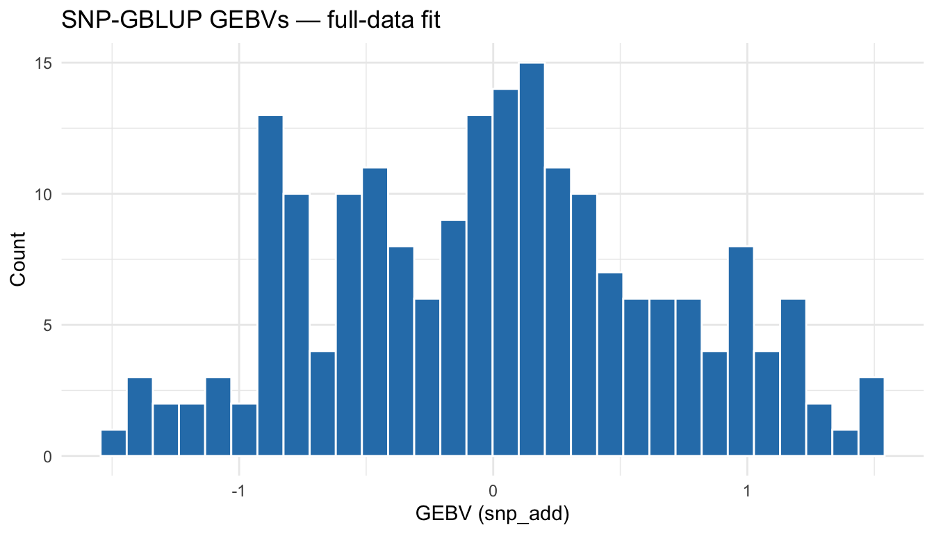

Predict on held-out candidates

The bundled demo provides a train_idx / test_idx split:

Code

train_ids <- d$pheno$id[d$train_idx]
test_ids  <- d$pheno$id[d$test_idx]

fit_train <- masreml(
  y       = y[train_ids],
  X       = X_fixed[d$train_idx, , drop = FALSE],
  markers = list(snp_add = d$snp[train_ids, , drop = FALSE]),
  trait   = "continuous",
  verbose = FALSE
)

pred <- predict(
  fit_train,
  markers_new   = list(snp_add = d$snp[test_ids, , drop = FALSE]),
  markers_train = list(snp_add = d$snp[train_ids, , drop = FALSE]),
  train_ids     = train_ids,
  test_ids      = test_ids,
  X_new         = X_fixed[d$test_idx, , drop = FALSE],
  y_new         = y[test_ids]
)

kable(as.data.frame(pred$metrics),
      digits  = 4,
      caption = "Held-out accuracy on the test split")

Held-out accuracy on the test split
R2	RMSE	accuracy	bias	AUC	r_MG
0.2368	1.3574	0.4866	1.3974	NA	0.7777

Cross-validation — `cv_masreml()`

cv_masreml() automates K-fold or family-based splits and refits the model on each training fold. Default is 5-fold random; pass scheme = "family" and a family-id vector for genuine candidate-selection accuracy.

Code

cv <- cv_masreml(
  y       = y,
  X       = X_fixed,
  markers = list(snp_add = d$snp),
  folds   = 5L,
  scheme  = "random",
  seed    = 123L
)

fold_tbl <- data.frame(
  fold     = seq_along(cv$accuracy_fold),
  accuracy = cv$accuracy_fold,
  bias     = cv$bias_fold
)
kable(fold_tbl, digits = 4, caption = "Per-fold test accuracy")

Per-fold test accuracy
	fold	accuracy	bias
fold1	1	0.2707	0.4167
fold2	2	0.3711	0.9222
fold3	3	0.4397	0.8650
fold4	4	0.6984	2.1233
fold5	5	0.5051	1.1072

Code

kable(data.frame(metric = c("Mean accuracy", "Mean bias"),
                 value  = c(cv$accuracy, cv$bias)),
      digits  = 4,
      caption = "Overall 5-fold CV summary")

Overall 5-fold CV summary
metric	value
Mean accuracy	0.4570
Mean bias	1.0869

Code

ggplot(fold_tbl, aes(x = factor(fold), y = accuracy)) +
  geom_col(fill = "#2c7fb8") +
  geom_hline(yintercept = mean(fold_tbl$accuracy),
             linetype = "dashed", colour = "red") +
  labs(x = "Fold", y = "Test accuracy (Pearson r)",
       title = "5-fold CV — SNP-GBLUP") +
  theme_minimal()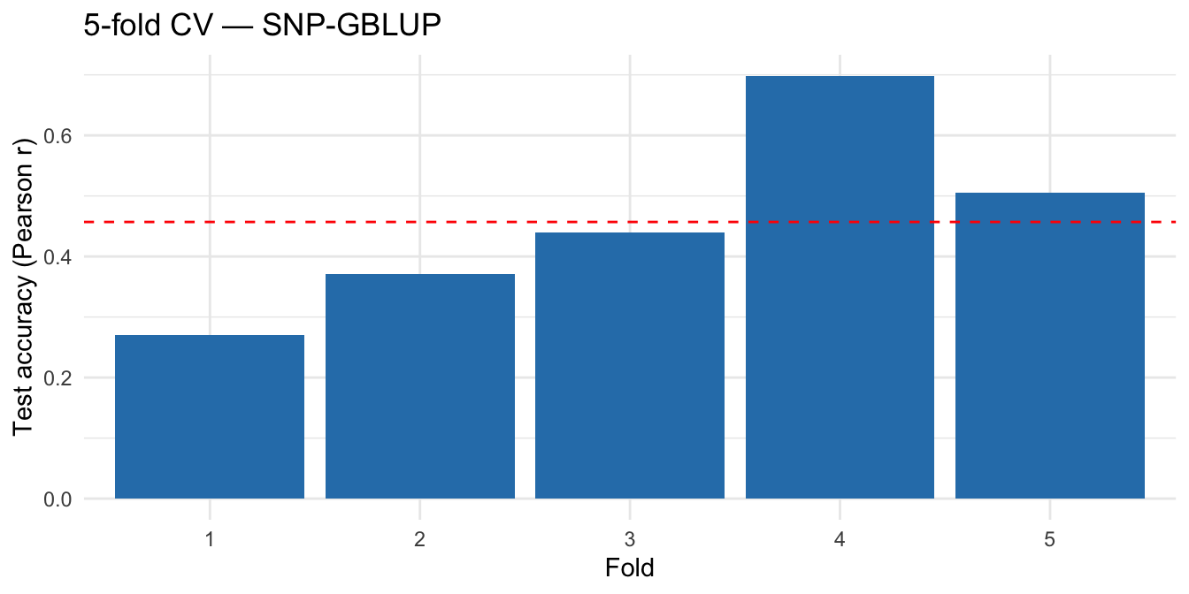

Binary trait

For 0/1 outcomes, set trait = "binary" and pick a link function. masreml runs a single-step Laplace approximation with the working response, returning the posterior mode of the liability-scale GEBV plus the fitted probability $\hat{p}_i$.

Code

y_bin <- setNames(d$pheno$y_bin_qtl_snp, d$pheno$id)

fit_bin <- masreml(
  y       = y_bin,
  X       = X_fixed,
  markers = list(snp_add = d$snp),
  trait   = "binary",
  link    = "logit",
  verbose = FALSE
)

summary(fit_bin)


══ masreml Summary ═══════════════════════════════════

Model:
  Call            : masreml(y = y_bin, X = X_fixed, markers = list(snp_add = d$snp), 
   Call            :     trait = "binary", link = "logit", verbose = FALSE)
  Individuals     : 200
  Components      : snp_add, residual
  Log-likelihood  : -302.6844
  Algorithm       : Laplace-1step (HE)
  Solver          : cholesky
  Converged       : TRUE (iterations = 1)

Variance Components:
 Component   Sigma2     H2 Proportion
   snp_add 0.730232 0.1816     0.1816
  residual 3.289868     NA     0.8184

Training Performance (observed/probability scale):
  AUC             : 0.8823
  R^2             : 0.4343
  RMSE            : 0.4159
  bias (slope)    : 2.171
  accuracy (r)    : 0.659

GEBV Summary:
 Component     Min Mean    Max    SD
   snp_add -1.1276    0 1.1707 0.612
     total -1.1276    0 1.1707 0.612

Binary Trait (GLMM Laplace):
  Link            : logit
  Prevalence      : 0.5000
  AUC             : 0.8823
  h2 (liability)  : 0.1816
  h2 (observed)   : 0.0887

Fitted Probabilities:
  Min=0.1959  Mean=0.4992  Max=0.7982  SD=0.1522

══════════════════════════════════════════════════════

fit_bin$h2 is reported on the liability scale (denominator $\sigma_u^2 + \pi^2/3$ for logit). Predictions return both the liability-scale GEBV and the observed-scale probability:

Code

pred_bin <- predict(fit_bin, y_new = y_bin)
kable(as.data.frame(pred_bin$metrics),
      digits  = 4,
      caption = "Training-set metrics, binary trait (AUC = discrimination)")

Training-set metrics, binary trait (AUC = discrimination)
R2	RMSE	accuracy	bias	AUC	scale
0.4343	0.4159	0.659	2.1709	0.8823	observed (probability scale)

Microhaplotype workflow

Switching from SNP to phased microhaplotype markers only changes the markers slot. Everything else — fitting, summary, prediction, cross-validation, binary trait — is identical.

Code

y_mh <- setNames(d$pheno$y_cont_qtl_mh, d$pheno$id)

fit_mhblup <- masreml(
  y       = y_mh,
  X       = X_fixed,
  markers = list(mh_add = d$mh),
  trait   = "continuous",
  verbose = FALSE
)
summary(fit_mhblup)


══ masreml Summary ═══════════════════════════════════

Model:
  Call            : masreml(y = y_mh, X = X_fixed, markers = list(mh_add = d$mh), 
   Call            :     trait = "continuous", verbose = FALSE)
  Individuals     : 200
  Components      : mh_add, residual
  Log-likelihood  : -162.6544
  Algorithm       : AI
  Solver          : cholesky
  Converged       : TRUE (iterations = 10)

Variance Components:
 Component   Sigma2     H2 Proportion
    mh_add 0.934674 0.4481     0.4481
  residual 1.151184     NA     0.5519

Training Performance:
  accuracy (r)    : 0.8639
  R^2             : 0.7463
  RMSE            : 0.8764
  bias (slope)    : 1.635

GEBV Summary:
 Component     Min Mean    Max     SD
    mh_add -1.8872    0 1.7011 0.7071
     total -1.8872    0 1.7011 0.7071

══════════════════════════════════════════════════════

Cross-validation on microhaplotype architecture:

Code

cv_mh <- cv_masreml(
  y       = y_mh,
  X       = X_fixed,
  markers = list(mh_add = d$mh),
  folds   = 5L,
  scheme  = "random",
  seed    = 123L
)

fold_mh_tbl <- data.frame(
  fold     = seq_along(cv_mh$accuracy_fold),
  accuracy = cv_mh$accuracy_fold,
  bias     = cv_mh$bias_fold
)
kable(fold_mh_tbl, digits = 4,
      caption = "5-fold CV — Microhaplotype-GBLUP")

5-fold CV — Microhaplotype-GBLUP
	fold	accuracy	bias
fold1	1	0.4778	1.3501
fold2	2	0.1582	0.2692
fold3	3	0.3197	0.9491
fold4	4	0.4712	1.6727
fold5	5	-0.0596	-0.1389

Binary trait on microhaplotype architecture:

Code

y_bin_mh <- setNames(d$pheno$y_bin_qtl_mh, d$pheno$id)

fit_bin_mh <- masreml(
  y       = y_bin_mh,
  X       = X_fixed,
  markers = list(mh_add = d$mh),
  trait   = "binary",
  link    = "logit",
  verbose = FALSE
)
summary(fit_bin_mh)


══ masreml Summary ═══════════════════════════════════

Model:
  Call            : masreml(y = y_bin_mh, X = X_fixed, markers = list(mh_add = d$mh), 
   Call            :     trait = "binary", link = "logit", verbose = FALSE)
  Individuals     : 200
  Components      : mh_add, residual
  Log-likelihood  : -244.4702
  Algorithm       : Laplace-1step (HE)
  Solver          : cholesky
  Converged       : TRUE (iterations = 1)

Variance Components:
 Component   Sigma2     H2 Proportion
    mh_add 0.730232 0.1816     0.1816
  residual 3.289868     NA     0.8184

Training Performance (observed/probability scale):
  AUC             : 0.8944
  R^2             : 0.4503
  RMSE            : 0.4062
  bias (slope)    : 1.981
  accuracy (r)    : 0.6711

GEBV Summary:
 Component     Min Mean    Max     SD
    mh_add -1.0096    0 1.0905 0.5384
     total -1.0096    0 1.0905 0.5384

Binary Trait (GLMM Laplace):
  Link            : logit
  Prevalence      : 0.5000
  AUC             : 0.8944
  h2 (liability)  : 0.1816
  h2 (observed)   : 0.0887

Fitted Probabilities:
  Min=0.1898  Mean=0.5000  Max=0.8203  SD=0.1698

══════════════════════════════════════════════════════

The W_αh coding (Da 2015) is constructed internally by masreml; no separate preprocessing call is needed when you go through masreml() directly. If you want to inspect or reuse the coded matrix, build it explicitly with masbayes::construct_wah_matrix() — see the masbayes tutorial and the Microhaplotype input page.

Working with the fit object

Beyond summary() and predict():

Code

kable(varcomp(fit_gblup),
      digits  = 4,
      caption = "Variance components (SNP-GBLUP)")

Variance components (SNP-GBLUP)
Component	Sigma2	H2	Proportion
snp_add	0.6559	0.3896	0.3896
residual	1.0276	NA	0.6104

Code

acc <- compute_accuracy(gebv = fit_gblup$total_gebv, y = y)
kable(as.data.frame(acc),
      digits  = 4,
      caption = "Training-set accuracy (SNP-GBLUP)")

Training-set accuracy (SNP-GBLUP)
r	slope	r_MG
0.7885	1.5434	NA

The full set of accessor methods:

Code

fit_gblup$gebv          # named list of per-component GEBVs
fit_gblup$total_gebv    # aggregated total GEBV vector
fit_gblup$converged     # convergence flag
fit_gblup$loglik        # REML log-likelihood
fit_gblup$n_iter        # iterations to convergence

See predict.masreml and evaluate_prediction for the full argument lists.

Setup

SNP workflow

Full-data fit — GBLUP

Predict on held-out candidates

Cross-validation — cv_masreml()

Binary trait

Microhaplotype workflow

Working with the fit object

See also

Cross-validation — `cv_masreml()`