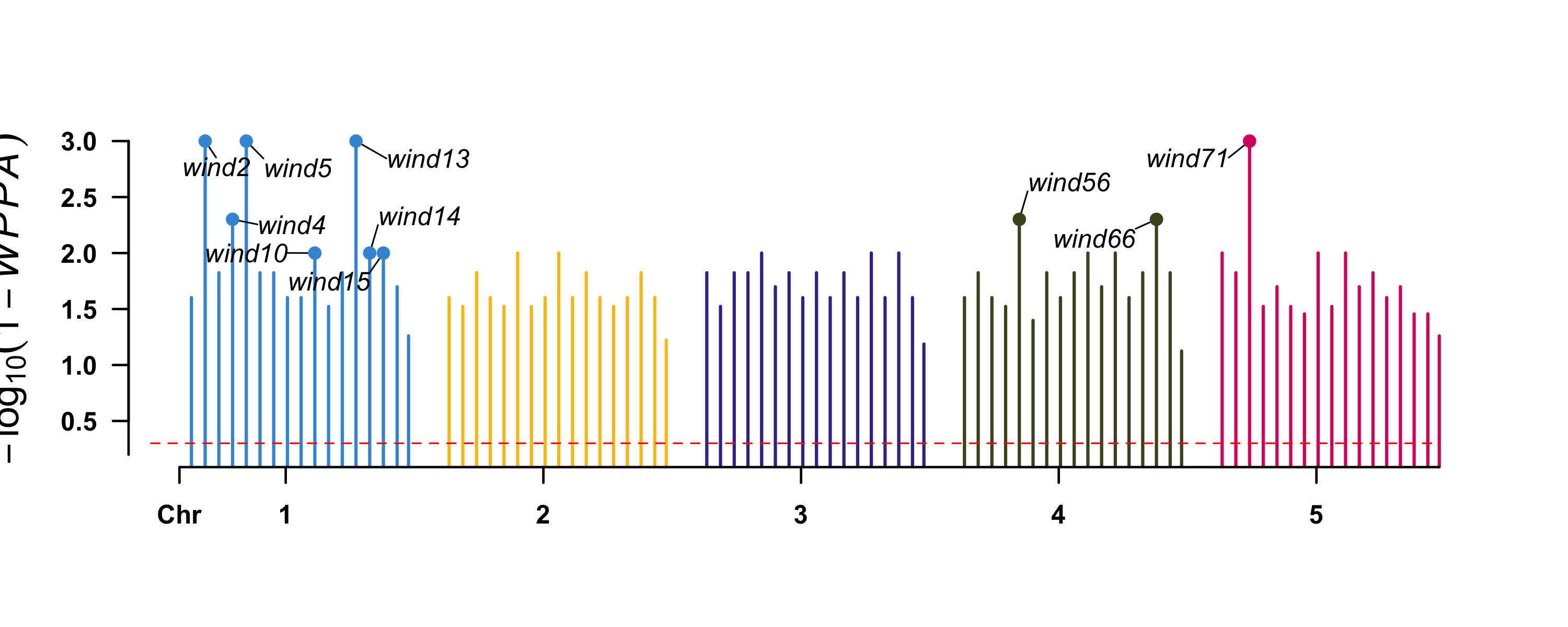
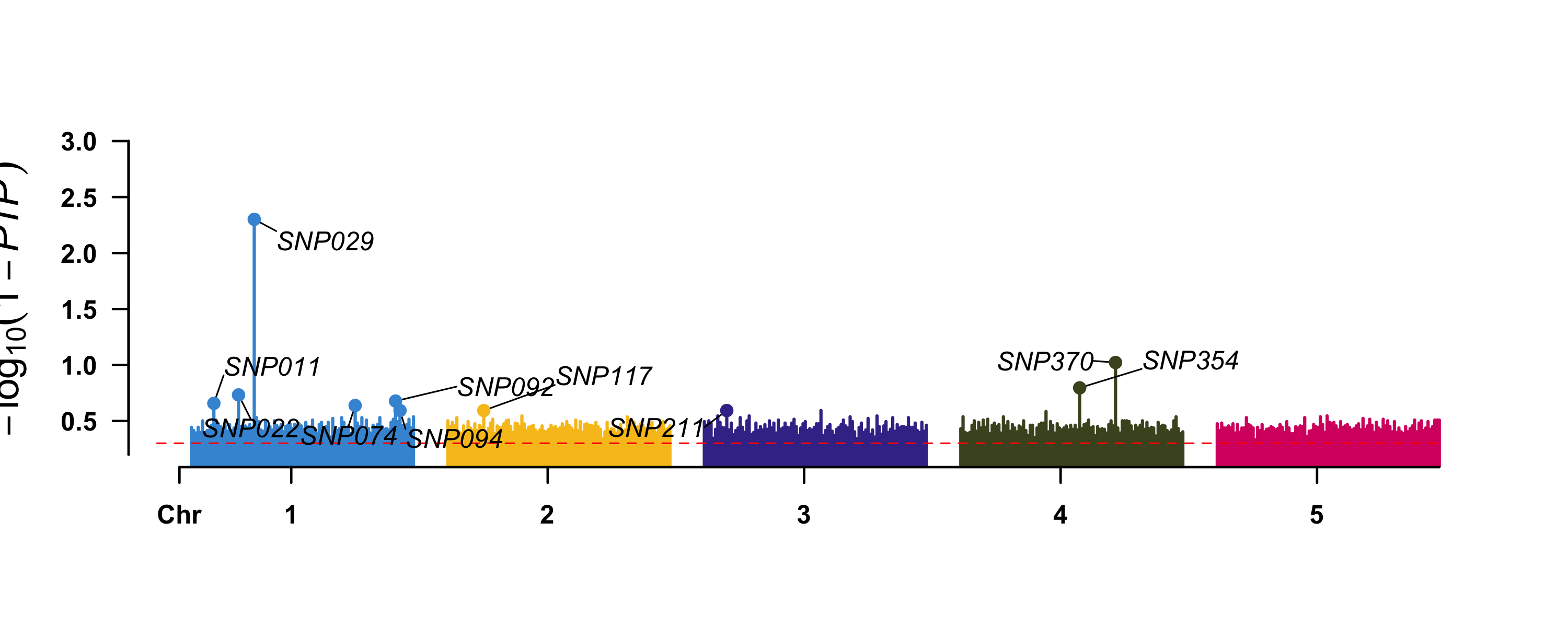
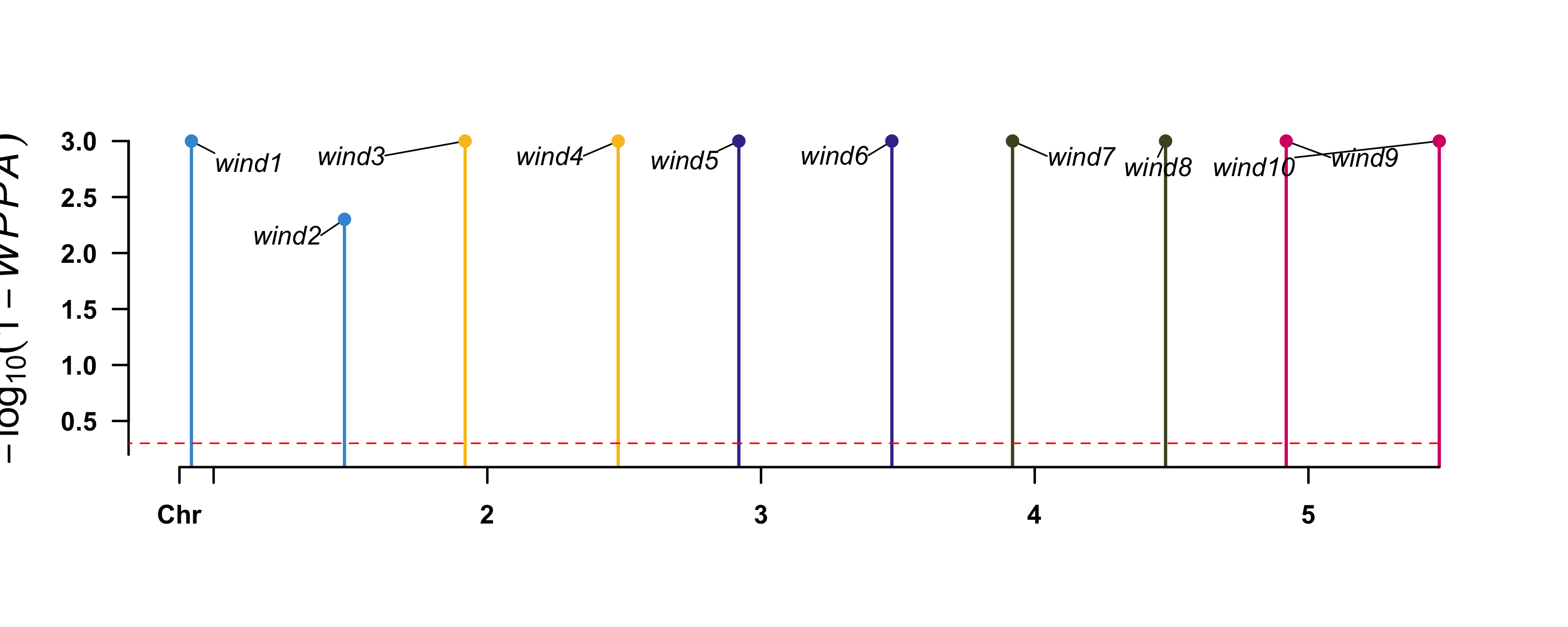
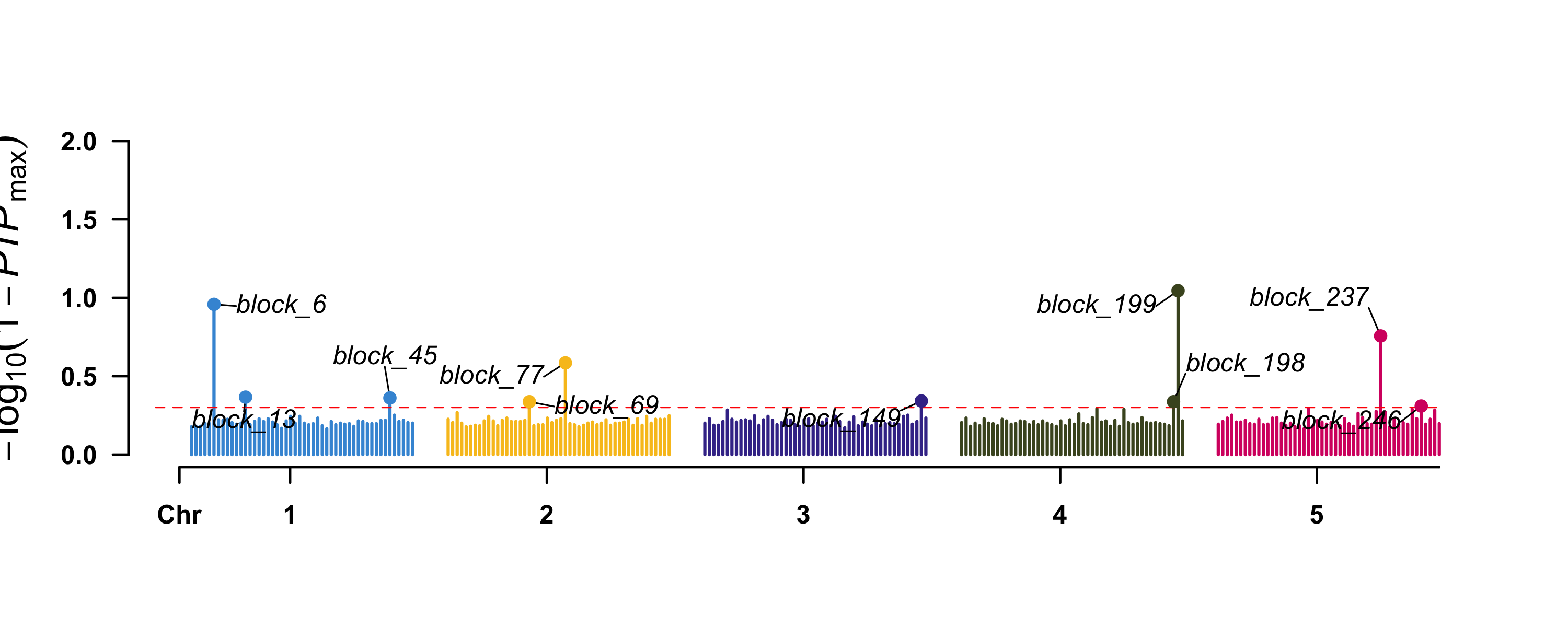
This tutorial extracts GWAS-style output from a BayesR MCMC fit: per-marker posterior inclusion probabilities (PIPs) and windowed posterior probabilities of association (WPPA) over physical-position windows. Both come for free from the posterior mixture-class samples — no separate scan is needed. The full source is adapted from masbayes/examples/04_gwas.R.
Important
MCMC required. PIPs and WPPA are derived from the posterior class trajectories (gamma_samples). The EM path of BayesR produces only MAP point estimates; passing method = "em" with a map argument errors out. Use method = "mcmc" for the entire workflow.
Important
BayesA has no equivalent. The scaled-\(t\) marginal places no mass on exactly zero, so PIP is not defined for BayesA. run_bayesa(..., map = ...) errors out by design. For frequentist GWAS, see the masreml page.
Setup
Code
library(masbayes)library(knitr)d<-load_data("large")# Tutorial-scale MCMC params; production should use n_iter = 20000+mcmc<-list(n_iter =2000L, n_burn =1000L, n_thin =5L, seed =42L)# Manhattan label cap. BayesR PIP/WPPA saturate on this demo data (most# markers exceed 0.5), so labelling every one above the threshold makes# CMplot's text placement hang. Label only the top-n peaks instead.n_label<-10L
Passing a map data frame plus either windsize (bp window) or windnum (consecutive-marker window) tells run_bayesr() to also compute PIPs and WPPA from the posterior samples. The Rust sampler is untouched; the extra output is post-processed on the R side from the existing gamma_samples matrix.
============================================================
 masbayes — BayesR with MCMC algorithm
============================================================
 Response type   : gaussian
 Observations    : n = 200, alleles p = 500
 Runtime         : 0.68 seconds

 Heritability (h2): 0.422

 MCMC Diagnostics
 ----------------------------------------
   Parameter             ESS    Geweke Z
   sigma2_e            110.0       -0.05
   mu                  200.0       -1.61
   beta (median)       200.0        0.06
 ----------------------------------------

 Run summary(fit) for full report.
============================================================
Step 3 — Top windows by WPPA
Code
top10_snp<-fit_snp$gwas[order(-fit_snp$gwas$WPPA), ][seq_len(10L), ]kable(top10_snp, digits =3, caption ="Top 10 SNP windows by WPPA")
Top 10 SNP windows by WPPA
Wind
Chr
N
Start
End
WPPA
2
wind2
1
6
1600000
2100000
1.000
5
wind5
1
6
3400000
3900000
1.000
13
wind13
1
6
8200000
8700000
1.000
71
wind71
5
6
2200000
2700000
1.000
4
wind4
1
6
2800000
3300000
0.995
56
wind56
4
6
3400000
3900000
0.995
66
wind66
4
6
9400000
9900000
0.995
10
wind10
1
6
6400000
6900000
0.990
14
wind14
1
6
8800000
9300000
0.990
15
wind15
1
6
9400000
9900000
0.990
WPPA is the fraction of posterior samples in which at least one marker inside the window had non-zero effect. It is the natural Bayesian analogue of the windowed-posterior column produced by masreml::run_gwas().
============================================================
 masbayes — BayesR with MCMC algorithm
============================================================
 Response type   : gaussian
 Observations    : n = 200, alleles p = 735
 Runtime         : 0.69 seconds

 Heritability (h2): 0.329

 MCMC Diagnostics
 ----------------------------------------
   Parameter             ESS    Geweke Z
   sigma2_e             83.8       -0.17
   mu                  200.0        1.41
   beta (median)       200.0        0.00
 ----------------------------------------

 Run summary(fit) for full report.
============================================================
Code
top10_mh<-fit_mh$gwas[order(-fit_mh$gwas$WPPA), ][seq_len(10L), ]kable(top10_mh, digits =3, caption ="Top 10 microhaplotype windows by WPPA")
Top 10 microhaplotype windows by WPPA
Wind
Chr
N
Start
End
WPPA
1
wind1
1
26
1050000
6050000
1.000
3
wind3
2
26
1050000
6050000
1.000
4
wind4
2
24
6250000
10850000
1.000
5
wind5
3
26
1050000
6050000
1.000
6
wind6
3
24
6250000
10850000
1.000
7
wind7
4
26
1050000
6050000
1.000
8
wind8
4
24
6250000
10850000
1.000
9
wind9
5
26
1050000
6050000
1.000
10
wind10
5
24
6250000
10850000
1.000
2
wind2
1
24
6250000
10850000
0.995
Note
Block-level PIP via max-per-block.fit_mh$pip_block is a union statistic (probability that at least one allele in the block is non-zero); on small block sizes this inflates and can put every block above the 0.5 threshold. We use max-per-block PIP instead — bounded by the maximum per-allele PIP within the block — which gives sharper QTL vs non-QTL discrimination.
The demo data ships with ground-truth QTL positions, so we can verify the BayesR scan recovers them — median PIP at true QTL should be substantially higher than at non-QTL markers.
Code
unit_index_mh<-match(attr(W_mh, "block_id"), map_mh$block_id)qtl_blocks<-unique(unit_index_mh[d$qtl$mh_idx])kable(data.frame( path =c("SNP (per-marker PIP)","Microhaplotype (per-block max PIP)"), pip_at_QTL =c(median(fit_snp$pip[d$qtl$snp_idx]),median(max_pip_block[qtl_blocks])), pip_non_QTL =c(median(fit_snp$pip[-d$qtl$snp_idx]),median(max_pip_block[-qtl_blocks]))), digits =3, caption ="Median PIP at true QTL vs non-QTL markers")
Median PIP at true QTL vs non-QTL markers
path
pip_at_QTL
pip_non_QTL
SNP (per-marker PIP)
0.66
0.645
Microhaplotype (per-block max PIP)
0.42
0.375
Accessing the fit object
Code
fit_snp$pip# per-marker PIP (length = ncol(W_snp))fit_snp$pip_block# per-block PIP (length = nrow(map))fit_snp$gwas# window data frame: Wind, Chr, N, Start, End, WPPAfit_snp$gwas_meta# call metadata: windsize, windnum, n_windows, ...fit_snp$beta_samples# full posterior trace, n_kept x ncol(W) (MCMC only)
See also
run_bayesr() — full signature including the map, windsize, windnum arguments
Theory overview — mixture prior, PIP diagnostics, \(\hat\pi_0\) interpretation