A genomic prediction model learns from a finite training sample, but breeders usually want its conclusions to apply to other individuals. A sample mean, marker effect, or prediction accuracy would change if a different set of individuals were measured. Statistical uncertainty describes this sample-to-sample variation. More records often improve precision, but a large sample from the wrong families, environments, or generations can still answer the wrong breeding question.
Population depends on the question
A biological population might mean all members of a herd, strain, or species. A statistical population is the collection or probability process about which an analysis seeks a conclusion. The target population must be stated more precisely than either label. It might consist of selection candidates from the same breeding programme next year, including the environments and management conditions in which they will be evaluated.
A sample is the set of individuals actually observed. In genomic prediction, the training sample contains the phenotypes and genotypes used to estimate a model. A sample is representative when its selection mechanism and biological structure retain the features relevant to the target population. Sample size alone cannot guarantee this. Two thousand close relatives from one environment may provide less information about an unrelated population than a smaller, deliberately diverse sample.
The examples below use the 200 simulated project individuals as an empirical population. Resampling from those records is a teaching device. It does not recreate the pedigree, meiosis, recombination, or environmental process that generated the original dataset.
A statistic varies across possible samples
A parameter such as a target-population mean is fixed but unknown under the frequentist framework used here. A statistic is calculated from a sample and therefore changes with the selected observations. The sampling distribution of a statistic describes its values over repeated samples drawn by the same procedure.
This differs from the phenotype distribution. One distribution contains individual phenotype values. The sampling distribution of the mean contains one mean from each possible sample. If independent observations come from a population with mean \(\mu\), variance \(\sigma^2\), and sample size \(n\), then
Because the population standard deviation \(\sigma\) is usually unknown, it is often replaced by the sample standard deviation \(s\). The square-root relation has an important consequence: doubling sample size does not halve the standard error. Under the same independent-sampling assumptions, four times as many observations are needed to halve it.
Manual example
The first five rounded project phenotypes from the descriptive-statistics page have mean \(\bar y=-1.4\) and sample standard deviation \(s=1.517\). Treating them temporarily as independent observations from a normal population gives
This interval is wide because five observations provide little information. It is only an arithmetic illustration. The first five rows were not obtained through a documented random-sampling design, and related individuals would violate the independence assumption. Those limitations prevent the interval from supporting a population claim here.
          mean standard_error          lower          upper
    -1.4000000      0.6782330     -3.2830767      0.4830767
Resampling the project phenotypes
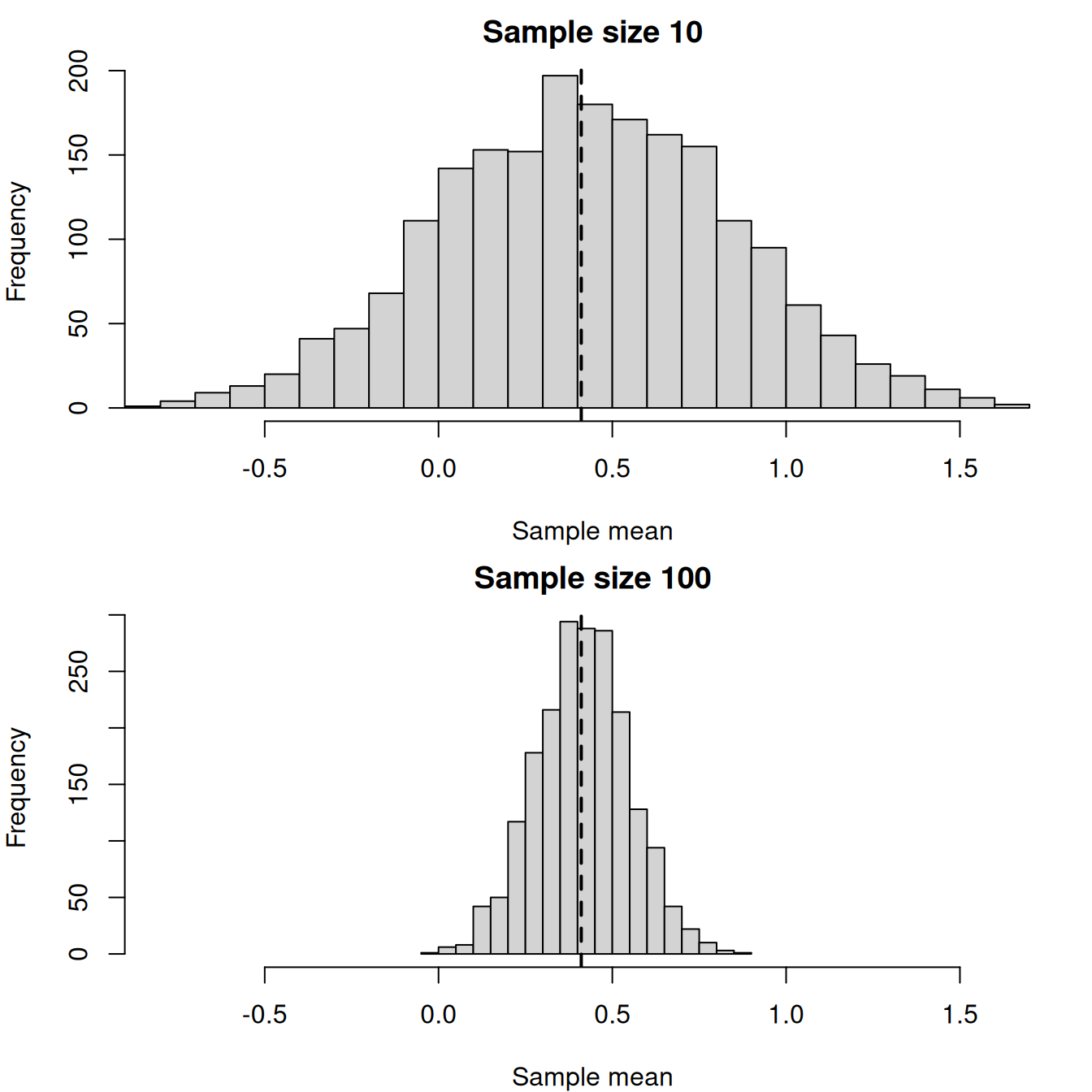
The following simulation repeatedly samples with replacement from the 200 raw continuous phenotypes. Each repeat produces one sample mean. The random seed makes the teaching result reproducible.
The 200 source phenotypes have standard deviation approximately 1.332. Across the resamples, means based on 10 records have standard deviation approximately 0.417, while means based on 100 records have standard deviation approximately 0.135. Increasing sample size narrows the sampling distribution of the mean; it does not change the spread of the 200 source phenotypes.
Figure 1: Sampling distributions from 2,000 resamples of the simulated project phenotypes. Both panels use the same horizontal scale. Means based on 100 observations cluster more tightly around the source-data mean than means based on 10 observations.
The observed ratio of the two simulation standard deviations is approximately 3.10, close to the theoretical ratio \(\sqrt{100/10}=\sqrt{10}\approx3.16\). Small differences are expected because the simulation uses a finite number of resamples.
Confidence intervals describe a procedure
A confidence interval combines an estimate with its sampling uncertainty. A 95% confidence procedure is designed so that, under its assumptions, about 95% of intervals calculated from repeated samples cover the fixed population parameter. Once one interval has been calculated, it either covers that parameter or it does not. The frequentist statement is not that there is a 95% probability that this one fixed interval contains the fixed parameter.
For an independent normal sample with unknown variance, the interval for a mean uses a Student-t critical value:
\[
\bar y \mathbin{\pm} t_{1-\alpha/2,n-1}\frac{s}{\sqrt n},
\]
where \(1-\alpha\) is the confidence level. Dependence among relatives, selective sampling, strong skew in a small sample, or unmodelled population structure can make this simple interval inappropriate. A genomic analysis must align its uncertainty calculation with its actual sampling and model structure.
An unbiased estimator is correct on average over repeated samples, but one realised estimate can still be far from the target. Precision describes the spread of the estimator’s sampling distribution. Larger samples often improve precision, but they do not repair bias caused by systematically missing a subpopulation or measuring the trait differently in training and deployment groups.
This distinction matters in breeding. A precisely estimated mean for one family may still be a biased estimate of the mean for all candidate families. Likewise, random cross-validation within a training population can estimate one prediction task precisely while giving an optimistic answer for future or unrelated candidates.
Exercises
Independent observations have standard deviation 10. Compare the standard error of the mean for sample sizes 25 and 100.
NoteSolution
For \(n=25\), the standard error is \(10/\sqrt{25}=2\). For \(n=100\), it is \(10/\sqrt{100}=1\). Quadrupling the sample size halves the standard error under the independence assumption.
A 95% confidence interval calculated from one sample is \((12,18)\). Is it correct to say that the fixed population mean has probability 0.95 of lying in this realised interval?
NoteSolution
No, not under the frequentist interpretation used here. The interval is the random object before sampling; the parameter is fixed. The 95% refers to the long-run coverage of the method over repeated samples generated under its assumptions.
A training sample contains many records but only from one family. Explain why increasing the number of records may narrow a standard error without making the sample representative of unrelated families.
NoteSolution
Additional records can reduce sample-to-sample variation for the family that was sampled. They do not add the allele frequencies, linkage patterns, or environments present in unobserved families. The estimate may therefore be precise for the sampled family but systematically unrepresentative of the broader target population.
Distinguish a parameter, a statistic, and a sampling distribution in the context of a training-sample mean.
NoteSolution
The target-population mean is a fixed but unknown parameter. A mean calculated from one training sample is a statistic. The sampling distribution describes the means that would result from repeated samples drawn by the same procedure.
The project resampling example compares means from samples of 10 and 100 records. What becomes narrower as sample size increases, and what does not?
NoteSolution
The sampling distribution of the mean becomes narrower, so its standard error decreases. The spread of the 200 source phenotypes does not change merely because larger resamples are taken.
A mean is estimated very precisely from a systematically unrepresentative training sample. Is the estimate necessarily unbiased for the target population? Explain.
NoteSolution
No. Precision is the spread of an estimator across repeated samples, whereas bias is its average difference from the target parameter. More records can narrow the sampling distribution without repairing systematic omission of a subpopulation or mismatch of measurement conditions.
Sampling uncertainty concerns the behaviour of one statistic across possible samples. The next mathematical topic examines how two variables vary together. Covariance and correlation provide the first tools for describing connections among phenotypes, breeding values, and later predictions.