Suppose a breeding candidate carries one copy of the alternative allele at a marker. That genotype describes the candidate, but it does not tell us whether the allele is rare or common among the animals from which candidates are selected. Answering that question requires a change of scale, from an individual genotype to counts across a defined population.
The population must be named because frequency is not an intrinsic property of an allele. The same allele can be common in one breed, uncommon in another, and absent from a third. It can also change in frequency between generations. This page develops the population quantities needed to describe those patterns and uses them to construct a reference model for genotype proportions.
From genotype counts to allele frequency
The previous page introduced a biallelic marker genotype as the number of copies of a chosen alternative allele: 0, 1, or 2. In a diploid population, each individual contributes two allele copies at an autosomal locus. If
\(n_0\) individuals have dosage 0,
\(n_1\) individuals have dosage 1, and
\(n_2\) individuals have dosage 2,
then the population sample contains \(n_0+n_1+n_2=N\) individuals and \(2N\) allele copies. The alternative allele occurs once in every dosage-1 genotype and twice in every dosage-2 genotype. Its count is therefore
\[
n_1 + 2n_2.
\]
The allele frequency is the proportion of all sampled allele copies that are the allele of interest. We will write the alternative-allele frequency as
\[
f_A = \frac{n_1 + 2n_2}{2N}.
\]
The reference-allele frequency is \(1-f_A\) because the locus is biallelic. The genotype frequencies are \(n_0/N\), \(n_1/N\), and \(n_2/N\). These two kinds of frequency answer different questions. Allele frequency counts copies of an allele, whereas genotype frequency counts individuals carrying each pair of alleles.
An allele is fixed in the sampled population when every sampled allele copy is the same, so its frequency is 1 and the other allele has frequency 0. Terms such as rare and common describe positions on the frequency scale, but their numerical boundaries depend on the population, sampling design, and analytical purpose. They should not be treated as universal biological categories.
A manual calculation for SNP007
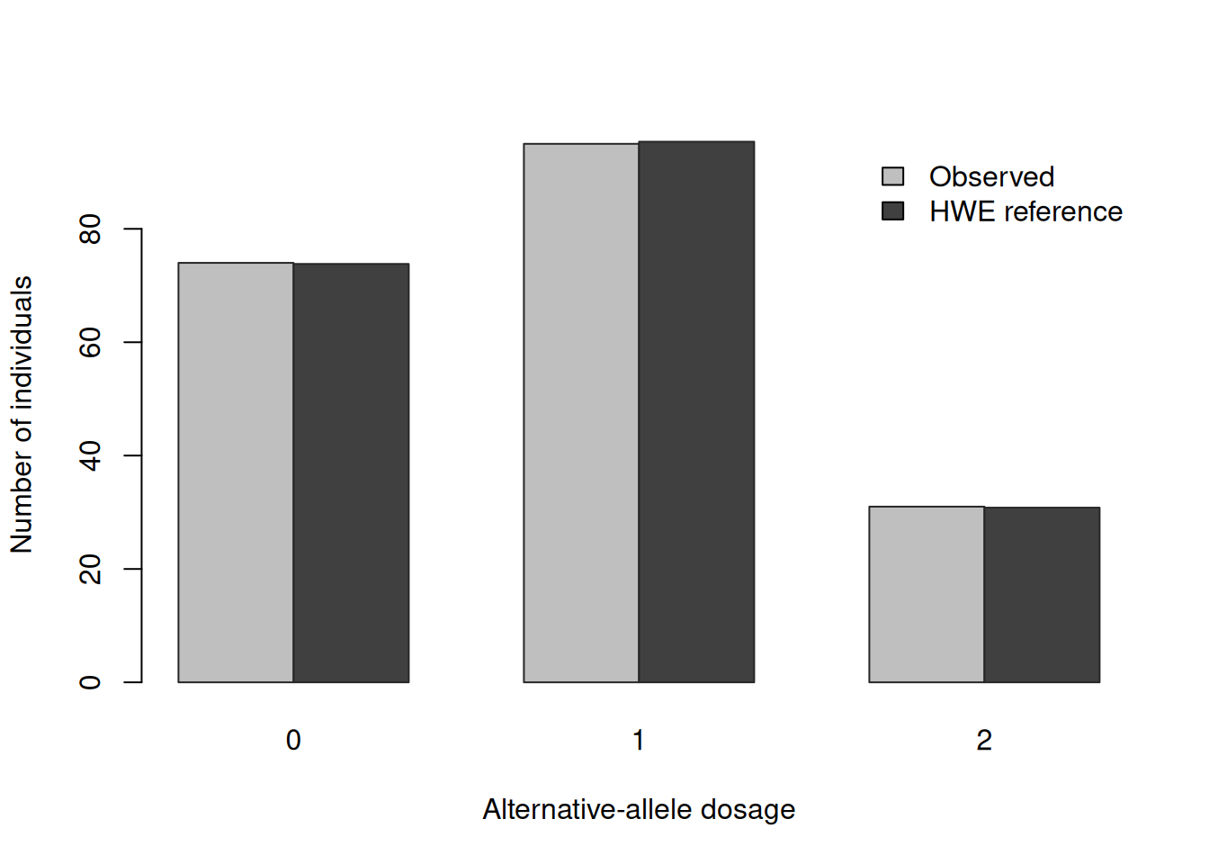
Among the 200 offspring in the project data, the observed dosage counts for SNP007 are 74, 95, and 31. The number of alternative-allele copies is
\[
95 + 2(31) = 157,
\]
and the total number of allele copies is
\[
2(200) = 400.
\]
Consequently,
\[
f_A = \frac{157}{400} = 0.3925,
\]
and the reference-allele frequency is \(1-0.3925=0.6075\). Notice that the alternative allele is not necessarily the less frequent allele. Reference and alternative remain coding labels, as explained on the variation and marker page.
Hardy-Weinberg proportions provide a reference
The Hardy-Weinberg model connects allele frequencies to expected genotype proportions. Consider an autosomal, biallelic locus in a diploid population. If alternative alleles occur in a fraction \(f_A\) of both male and female gametes and gametes combine at random with respect to this locus, the possible unions give
The factor 2 in the heterozygous proportion appears because the alternative allele can come from either gamete. Random union of gametes produces these genotype proportions in one generation. For allele frequencies themselves to remain constant across generations, the classical equilibrium model also assumes no selection, migration, or mutation and a population large enough that random sampling does not appreciably change frequencies.
For SNP007, multiplying the three proportions by \(N=200\) gives
Expected counts need not be whole numbers. They describe the average pattern implied by the model, not a second set of observed individuals.
Verify the calculation in R
The same calculation can be performed directly from the project genotype matrix. Taking the mean dosage counts alternative alleles per individual; dividing by two converts that mean to a proportion of allele copies.
The R result matches the manual calculation: the observed counts are 74, 95, and 31, while the Hardy-Weinberg reference counts are approximately 73.8, 95.4, and 30.8.
Observed genotype counts at SNP007 and counts calculated from Hardy-Weinberg reference proportions. The close bars describe this marker in this sample only.
Why population frequencies and proportions change
Hardy-Weinberg proportions are useful precisely because real populations can depart from the reference for interpretable reasons. Several mechanisms must be distinguished because they do not all have the same immediate effect.
Mutation creates new sequence variants. At an individual locus its per-generation contribution is usually small, but mutation is the ultimate source of alleles on which other processes act.
Selection occurs when genotypes differ in survival or reproductive contribution. In a breeding programme, deliberate choice of parents is a form of selection. If the selected trait is influenced by a locus, or by a linked locus inherited with it, allele frequencies can change between the candidate and offspring generations.
Genetic drift is random change in allele frequency caused by finite sampling of parents and gametes. Even equally fit alleles are not guaranteed to contribute the same number of copies to the next generation. Drift is stronger when relatively few individuals contribute genetically.
Migration, also called gene flow in population genetics, moves allele copies between populations when immigrants reproduce. Introducing animals or germplasm from another breeding population can therefore change local allele frequencies. The direction and magnitude depend on the migrants’ frequencies and their reproductive contribution.
Non-random mating changes which allele copies occur together in individuals. Mating relatives, for example, tends to increase homozygosity and reduce heterozygosity relative to random mating. It can change genotype proportions immediately even when it does not, by itself, change the allele frequency in that generation.
Population structure exists when the sampled individuals come from subpopulations with different ancestry or allele frequencies. Pooling such groups and calculating one frequency can produce a heterozygote deficit relative to the pooled Hardy-Weinberg expectation, even if each group is close to its own reference proportions. Family groups are also a form of sampling structure because relatives share segments inherited from recent ancestors.
The effective population size, written \(N_e\), describes the size of an idealised population that would experience genetic drift at the same rate as the population under study. It is not simply the number of animals alive or genotyped. Unequal numbers of breeding males and females, unequal family sizes, and large differences in reproductive success can make \(N_e\) much smaller than the census size. This distinction matters in breeding programmes because using many candidates does not prevent drift if only a small number become parents.
Agreement is not proof of equilibrium or independence
The close observed and reference counts for SNP007 show that one summary of this marker is numerically consistent with Hardy-Weinberg proportions. They do not prove that the breeding population satisfies every classical assumption. A similar match can occur by chance, and a single-locus comparison cannot diagnose selection, migration, genotyping error, or population structure on its own.
The sampling design is especially important here. The 200 records are offspring from ten full-sib families, with 20 offspring per family. Siblings share parents and are therefore not independent draws from a freely mating population. Any formal test or downstream model must account for the design rather than treating numerical agreement at one marker as evidence of independent sampling.
Later, the Genomic prediction section will use allele frequencies to centre and sometimes scale marker dosages. This page stops at their biological and population interpretation so that the modelling operation is introduced where its purpose can be made explicit.
Exercises
A sample of 20 individuals has genotype counts \(n_0=8\), \(n_1=10\), and \(n_2=2\). Calculate the alternative-allele count and frequency.
NoteSolution
The alternative-allele count is \(10+2(2)=14\). There are \(2(20)=40\) allele copies, so \(f_A=14/40=0.35\).
For \(N=100\) and \(f_A=0.30\), calculate the Hardy-Weinberg reference counts for dosages 0, 1, and 2.
NoteSolution
The proportions are \(0.70^2=0.49\), \(2(0.30)(0.70)=0.42\), and \(0.30^2=0.09\). Multiplying by 100 gives expected counts of 49, 42, and 9.
Suppose relatives mate more often than expected, but no allele copies enter or leave the population. What can change immediately?
NoteSolution
The pairing of alleles into genotypes can change, commonly producing more homozygotes and fewer heterozygotes. The allele frequency need not change in that generation because the same allele copies are being paired differently.
Explain the difference between allele frequency and genotype frequency at a biallelic autosomal locus. Which quantity counts allele copies rather than individuals?
NoteSolution
Allele frequency is the proportion of all allele copies that are a chosen allele, whereas genotype frequencies are the proportions of individuals with dosages 0, 1, and 2. Allele frequency counts copies, so its denominator is \(2N\) for \(N\) diploid individuals.
A breeding population has many animals alive but only a few parents that contribute very unequally to the next generation. What does this imply about effective population size and genetic drift?
NoteSolution
Its effective population size can be much smaller than its census size. The idealised effective size reflects the rate of drift, and unequal reproductive contribution increases that rate because relatively few parents transmit the alleles represented in the next generation.
Observed counts at one marker are close to its Hardy-Weinberg reference counts in the project data. Why does this not prove equilibrium or that the 200 offspring are independent draws from a freely mating population?
NoteSolution
A close numerical match can occur by chance and one locus cannot diagnose all model assumptions. The records are offspring from ten full-sib families, so siblings share parents and are not independent draws. Selection, migration, genotyping error, and population structure also cannot be ruled out from this one comparison.
Allele frequencies describe one locus at a time. The next question is how alleles at different loci become associated on chromosomes and across a population.